library(ggplot2)
library(patchwork)

te_paper  <- "#f5f4ee"
te_ink    <- "#16241d"
te_body   <- "#2c3a31"
te_forest <- "#275139"
te_rust   <- "#b5534e"
te_gold   <- "#c9b458"
te_line   <- "#dad9ca"

theme_datasheet <- function() {
  theme_minimal(base_size = 12) +
    theme(plot.background  = element_rect(fill = te_paper, colour = NA),
          panel.background = element_rect(fill = te_paper, colour = NA),
          panel.grid.major = element_line(colour = te_line, linewidth = 0.3),
          panel.grid.minor = element_blank(),
          text             = element_text(colour = te_body),
          plot.title       = element_text(colour = te_ink, face = "bold"),
          plot.subtitle    = element_text(colour = te_body),
          axis.text        = element_text(colour = te_body))
}

psi0    <- 0.5
lam_lo  <- 1
lam_hi  <- 2
budget  <- 100
k_std <- 4What a detection time is worth
R
occupancy
survey design
detection probability
ecology tutorial
Occupancy visits record only detected or not detected, discarding the detection times. Measure in R, from exact Fisher information, what that choice costs.
A surveyor stands at a forest point for one hour and listens. The species calls at twelve minutes, again at thirty four, and once more at fifty one. What reaches the datasheet is four boxes, one per quarter of an hour, three of them ticked. The three times are written nowhere.
That datasheet is the standard input to a single season occupancy model: a count of detections out of four at each of a hundred points, from which occupancy and per visit detection are estimated jointly. It is also a summary, because the underlying observation was a sequence of encounter times and the boxes keep only whether each quarter hour contained at least one. What this post measures is what the discarded times were worth: not whether a continuous record is more informative, which it cannot fail to be, but how much more, expressed as a standard error on occupancy under a fixed field budget.
This sits next to two existing posts. The one on how many visits an occupancy survey needs treats each visit as a separate trip, so K visits cost K times as much and the design question is a budget question. The one on fitting the single season likelihood builds the estimator this post takes as given. Here the hour of searching is held fixed for the first half, and the only choice is how finely it is written down, so every slicing of that hour costs the same. That makes the recording question an information question with an exact answer. The second half lets the hour itself move, and that turns out to be worth more than any of the recording choices.
An hour of listening, and three ways to write it down
The setting is fixed for now. Occupancy is psi = 0.5. At an occupied site, encounters arrive as a Poisson process with rate lambda per hour, and the surveyor searches for one hour. At an empty site nothing is ever detected, so there are no false positives. The total budget is one hundred search hours, and the three designs spend it differently. The one hour window is a stipulation and not a result, and the later sections take it back.
The first design writes down every encounter time, minute by minute. The second ticks k_std boxes of fifteen minutes each, so a box says only whether that quarter of an hour held at least one encounter. The third stops the moment the species is first encountered and moves on, which is the removal or time to detection design of Garrard et al. 2008 and Bornand et al. 2014.
The detection times add nothing the count does not carry
Write the likelihood for the first design. At an occupied site the density of a realisation of a homogeneous Poisson process with nn points on an hour of watching is exp(-lambda) * lambda^nn. The individual times appear nowhere in that expression: only how many there were. So the full record and a tally of encounters carry exactly the same information about lambda, and the same about occupancy, which is the first thing worth knowing before designing a stopwatch protocol.
Sites with no encounter are the usual mixture. Either the site is occupied and the process produced nothing in the hour, or it is empty.
info_full <- function(psi, lam) {
  nn <- 0:(qpois(1 - 1e-12, lam) + 40); a0 <- psi * exp(-lam) + (1 - psi)
  prb <- ifelse(nn == 0, a0, psi * dpois(nn, lam))
  sc_psi <- ifelse(nn == 0, (exp(-lam) - 1) / a0, 1 / psi)
  sc_lam <- ifelse(nn == 0, -psi * exp(-lam) / a0, nn / lam - 1)
  matrix(c(sum(prb * sc_psi^2), sum(prb * sc_psi * sc_lam),
           sum(prb * sc_psi * sc_lam), sum(prb * sc_lam^2)), 2, 2)
}
se_psi <- function(im, n_site) sqrt(solve(im)[1, 1] / n_site)
se_full_lo <- se_psi(info_full(psi0, lam_lo), budget)
se_full_hi <- se_psi(info_full(psi0, lam_hi), budget)
c(lam_lo = se_full_lo, lam_hi = se_full_hi)
lam_lo lam_hi
0.09726796 0.06032576 Those two numbers are the reference the rest of the post is measured against. With 100 sites each watched for a full hour, and every encounter time in hand, occupancy carries a standard error of 0.0973 when the rate is one encounter per hour and 0.0603 when it is two. No design that watches the same hour and records anything less can do better than that. Where the coarser designs lose, and where they do not, is the subject of the next section.
Four binary slices cost eight per cent of the standard error
The k_std box datasheet is the standard occupancy design applied inside a single hour. A slice of length one over K contains at least one encounter with probability 1 - exp(-lambda / K), and the number of ticked boxes at an occupied site is binomial. The Fisher information is the one the design post on this site already uses, with detection per visit written as a function of the rate.
info_slice <- function(psi, lam, kk) {
  pp <- 1 - exp(-lam / kk); dd <- 0:kk; a0 <- psi * (1 - pp)^kk + (1 - psi)
  prb <- ifelse(dd >= 1, psi * choose(kk, dd) * pp^dd * (1 - pp)^(kk - dd), a0)
  sc_psi <- ifelse(dd >= 1, 1 / psi, ((1 - pp)^kk - 1) / a0)
  sc_p   <- ifelse(dd >= 1, dd / pp - (kk - dd) / (1 - pp),
                   psi * (-kk) * (1 - pp)^(kk - 1) / a0)
  matrix(c(sum(prb * sc_psi^2), sum(prb * sc_psi * sc_p),
           sum(prb * sc_psi * sc_p), sum(prb * sc_p^2)), 2, 2)
}
info_slice_lam <- function(psi, lam, kk) {   # the same design, in occupancy and rate
  im <- info_slice(psi, lam, kk); jj <- exp(-lam / kk) / kk
  matrix(c(im[1, 1], jj * im[1, 2], jj * im[1, 2], jj^2 * im[2, 2]), 2, 2)
}
se_k4_lo <- se_psi(info_slice(psi0, lam_lo, k_std), budget)
se_k4_hi <- se_psi(info_slice(psi0, lam_hi, k_std), budget)
infl_lo <- 100 * (se_k4_lo / se_full_lo - 1); infl_hi <- 100 * (se_k4_hi / se_full_hi - 1)
more_lo <- 100 * ((se_k4_lo / se_full_lo)^2 - 1); more_hours <- budget * more_lo / 100
im_full <- info_full(psi0, lam_lo); im_k2 <- info_slice_lam(psi0, lam_lo, 2)
im_k4 <- info_slice_lam(psi0, lam_lo, k_std)
occ_diag <- im_full[1, 1]; off_diag <- im_full[1, 2]
agree_all <- max(abs(c(im_k2[1, 1], im_k4[1, 1]) - occ_diag),
                 abs(c(im_k2[1, 2], im_k4[1, 2]) - off_diag))
rate_k2 <- im_k2[2, 2]; rate_k4 <- im_k4[2, 2]; rate_full <- im_full[2, 2]
blank_prob <- exp(-lam_lo); psi_grid <- seq(0.05, 0.95, 0.05)
se_by_psi <- vapply(psi_grid, function(a) se_psi(info_slice(a, lam_lo, k_std), budget), 0)
psi_worst <- psi_grid[which.max(se_by_psi)]; se_worst <- max(se_by_psi)
c(se_k4_lo = se_k4_lo, rate_k4 = rate_k4, rate_full = rate_full, agree = agree_all)
se_k4_lo rate_k4 rate_full agree
1.053015e-01 3.056307e-01 3.655293e-01 1.110223e-16 Four boxes give 0.1053 at a rate of one per hour against the 0.0973 of the full record, which is 8.3 per cent more standard error. At a rate of two the gap shrinks to 2.4 per cent. Buying that precision back with extra sites, rather than with a stopwatch, takes 17 per cent more of them: 17 extra hours on top of 100. That is the price of the timestamps, and whether a stopwatch protocol is worth building depends on whether it costs less than that.
It is worth being exact about where the loss comes from, because the obvious answer is wrong. It does not come from the sites that produce nothing. An occupied site stays blank when the hour contains no encounter at all, which has probability 0.3679 whatever the datasheet looks like, since no coarsening of a record can turn an empty hour into a detection. Put every design in the same two parameters and the information matrices differ in one entry only: the occupancy diagonal is 1.8485 and the occupancy by rate off diagonal is 0.5379 under two slices, four slices and the full record alike, agreeing to within floating-point rounding (the printed agree). What changes is the rate diagonal, 0.2509 at two slices, 0.3056 at four and 0.3655 with every time in hand. Coarsening costs nothing on the blank sites and nothing on the occupancy score; it costs information about the encounter rate, which reaches occupancy only through the off diagonal that the inverse has to carry. That is why so large a change in the record moves the occupancy standard error so little.
The sweep flattens onto a bound, and it flattens early
Nothing stops a surveyor from ticking finer boxes. Eight boxes of seven and a half minutes each cost the same hour, and so do sixty boxes of one minute each. The sequence has to approach the full record, because in the limit a box is either empty or holds one encounter at a known minute, and the interesting part is how fast it gets there and where it stops.
k_grid <- 2:30
sweep_dat <- data.frame(kk = rep(k_grid, 2), lam = rep(c(lam_lo, lam_hi), each = length(k_grid)))
sweep_dat$se <- mapply(function(a, b) se_psi(info_slice(psi0, b, a), budget),
                       sweep_dat$kk, sweep_dat$lam)
sweep_dat$rate <- factor(sprintf("lambda = %g per hour", sweep_dat$lam))
bound_dat <- data.frame(se = c(se_full_lo, se_full_hi),
  rate = factor(sprintf("lambda = %g per hour", c(lam_lo, lam_hi))))

k_fine <- 2:400
fine_lo <- vapply(k_fine, function(a) se_psi(info_slice(psi0, lam_lo, a), budget), 0)
fine_hi <- vapply(k_fine, function(a) se_psi(info_slice(psi0, lam_hi, a), budget), 0)
first_within <- function(ses, bound, tol) k_fine[which(ses / bound - 1 < tol)[1]]
k5_lo <- first_within(fine_lo, se_full_lo, 0.05); k1_lo <- first_within(fine_lo, se_full_lo, 0.01)
k5_hi <- first_within(fine_hi, se_full_hi, 0.05)
k_top <- max(k_fine); still_over <- 100 * (fine_lo[length(fine_lo)] / se_full_lo - 1)
gap_k8 <- 100 * (se_k4_lo - se_psi(info_slice(psi0, lam_lo, 2 * k_std), budget)) /
  (se_k4_lo - se_full_lo); mono_ok <- all(diff(fine_lo) < 0)
c(k5_lo = k5_lo, k5_hi = k5_hi, k1_lo = k1_lo, monotone = mono_ok)
k5_lo k5_hi k1_lo monotone
7 3 27 1 ggplot(sweep_dat, aes(kk, se, colour = rate)) +
geom_hline(data = bound_dat, aes(yintercept = se, colour = rate),
linetype = "22", linewidth = 0.6) +
geom_line(linewidth = 0.9) +
geom_point(size = 1.7) +
geom_point(data = subset(sweep_dat, kk == k_std), colour = te_gold, size = 3.4) +
geom_text(data = bound_dat, aes(x = max(k_grid), y = se, colour = rate),
label = "continuous time bound", hjust = 1, vjust = 1.8, size = 3.2,
show.legend = FALSE) +
scale_colour_manual(values = c(te_forest, te_rust), name = NULL) +
scale_x_continuous(breaks = c(2, 4, 8, 12, 16, 20, 24, 28)) +
scale_y_continuous(expand = expansion(mult = c(0.14, 0.05))) +
labs(x = "binary slices per hour (K)", y = "standard error of occupancy",
title = "Finer boxes stop paying quickly",
subtitle = "gold points: the four box datasheet") +
theme_datasheet() +
theme(legend.position = "bottom")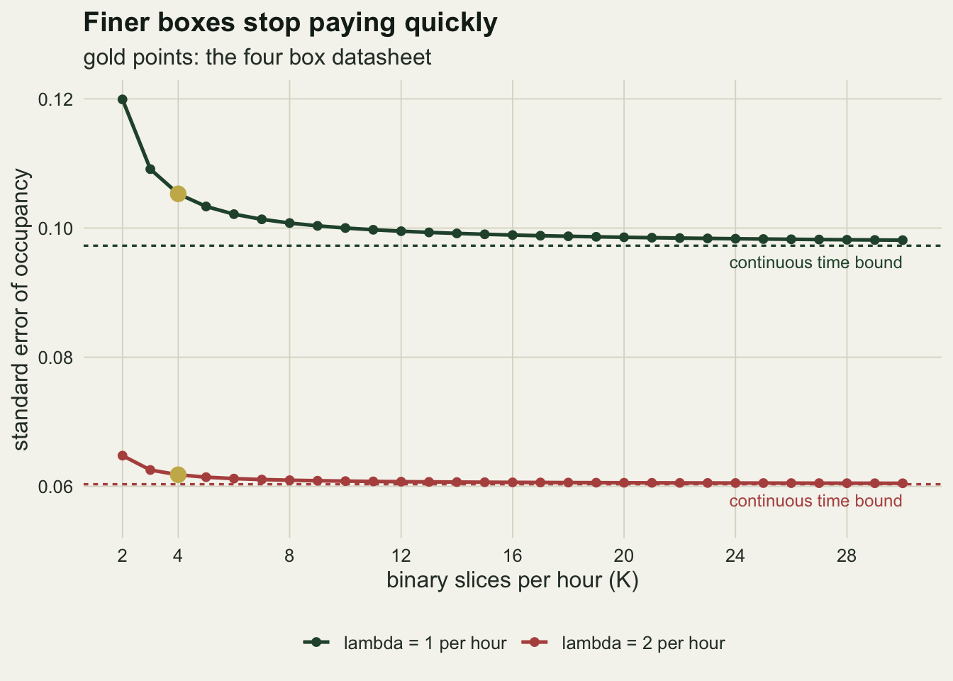
The curve for the lower rate reaches within five per cent of the bound at 7 slices and within one per cent at 27. At the higher rate five per cent arrives at 3 slices. Past that the curve is doing almost nothing: at 400 slices, which is a box every nine seconds, the standard error is still 0.06 per cent above the bound and falling by amounts no field programme could notice. The approach is monotone from above and never crosses.
A surveyor who was about to build a protocol with a stopwatch, a voice recorder and a transcription step is buying, at best, the gap between the four box number and the dashed line. Cutting the hour into eight boxes instead of four costs no extra field time, needs no new equipment, and closes 56 per cent of that gap on its own.
Stopping at the first detection buys sites and sells rate information
The removal design does not summarise the hour. It shortens it: search until the species is found, record when, and leave. That changes the cost per site as well as the record, so it must be compared on the budget rather than on the site count. Expected search time at an occupied site is (1 - exp(-lambda)) / lambda hours, and an empty site consumes the whole hour because nothing ever stops the search.
cost_stop <- function(psi, lam) psi * (1 - exp(-lam)) / lam + (1 - psi)
info_stop <- function(psi, lam) {
  a0 <- psi * exp(-lam) + (1 - psi)
  dens <- function(tt) psi * lam * exp(-lam * tt)
  ipp <- integrate(function(tt) dens(tt) / psi^2, 0, 1)$value + (1 - exp(-lam))^2 / a0
  ipl <- integrate(function(tt) dens(tt) * (1 / psi) * (1 / lam - tt), 0, 1)$value -
         psi * exp(-lam) * (exp(-lam) - 1) / a0
  ill <- integrate(function(tt) dens(tt) * (1 / lam - tt)^2, 0, 1)$value +
    (psi * exp(-lam))^2 / a0
  matrix(c(ipp, ipl, ipl, ill), 2, 2)
}

cost_lo <- cost_stop(psi0, lam_lo); n_stop_lo <- budget / cost_lo
cost_hi <- cost_stop(psi0, lam_hi); n_stop_hi <- budget / cost_hi
se_stop_lo <- se_psi(info_stop(psi0, lam_lo), n_stop_lo)
se_stop_hi <- se_psi(info_stop(psi0, lam_hi), n_stop_hi)
im_stop <- info_stop(psi0, lam_lo); rate_stop <- im_stop[2, 2]; rate_share <- 100 * rate_stop / rate_full
cor_of <- function(im) { vv <- solve(im); vv[1, 2] / sqrt(vv[1, 1] * vv[2, 2]) }
cor_stop <- cor_of(im_stop); cor_full <- cor_of(im_full)
cross_lam <- uniroot(function(lam) se_psi(info_stop(psi0, lam), budget / cost_stop(psi0, lam)) -
  se_psi(info_slice(psi0, lam, k_std), budget), c(1.2, 5))$root
n_lo_use <- as.integer(floor(n_stop_lo))
c(cost_lo = cost_lo, n_stop_lo = n_stop_lo, se_stop_lo = se_stop_lo, rate_stop = rate_stop)
cost_lo n_stop_lo se_stop_lo rate_stop
0.8160603 122.5399674 0.1788161 0.1815896 At the lower rate a site costs 0.816 hours instead of one, so the same budget reaches 122.5 sites instead of 100. The extra sites do not pay for the record: the standard error is 0.1788 against 0.1053 for four boxes on 100 sites. The blank sites are not the reason. They are the same blank sites with the same probability 0.3679, and the design has the same occupancy diagonal and off diagonal as every other design here. The reason is that it throws away every encounter after the first, which leaves a rate diagonal of 0.1816 against the 0.3655 of the full hour, or 50 per cent of it. With that little rate information the two parameters are hard to tell apart: the implied correlation between the occupancy and rate estimates is -0.928 here against -0.654 for the full record.
At the higher rate the gap closes. The saving is larger, 139.6 sites fit in the budget, and the standard error comes to 0.0618, matching the four box design’s 0.0618 to four decimals. The crossing is at a rate of 2.00 encounters per hour. That crossing is a real feature of the arithmetic, and it is also the point at which this comparison should be distrusted, because one hour of searching has been imposed on a design whose whole idea is not to search for a fixed time.
The search window decides more than the datasheet does
The window is the one design parameter held constant so far, and it is the only one the three designs do not share by construction. Let it be W hours. A slice design cuts W into k_std boxes, so a box holds an encounter with probability one minus exp(-lambda * W / K), and a site costs W. A removal design censors at W, so a site costs psi * (1 - exp(-lambda * W)) / lambda + (1 - psi) * W. In all three cases the rate and the window enter the information only through their product, so the functions already written can be reused with the rate rescaled.
se_slice_w <- function(lam, ww, trav = 0)
  se_psi(info_slice(psi0, lam * ww, k_std), budget / (ww + trav))
se_full_w <- function(lam, ww, trav = 0)
  se_psi(info_full(psi0, lam * ww), budget / (ww + trav))
cost_stop_w <- function(lam, ww) ww * cost_stop(psi0, lam * ww)
se_stop_w <- function(lam, ww, trav = 0)
  se_psi(info_stop(psi0, lam * ww), budget / (cost_stop_w(lam, ww) + trav))
stopifnot(all.equal(se_slice_w(lam_lo, 1), se_k4_lo), all.equal(se_full_w(lam_lo, 1), se_full_lo),
          all.equal(se_stop_w(lam_lo, 1), se_stop_lo))

best_w <- function(fn, hi = 30) {           # and check the minimum is inside the bracket
  op <- optimize(fn, c(0.05, hi))
  stopifnot(op$minimum > 0.06, op$minimum < hi - 0.5)
  unname(c(op$minimum, op$objective))
}
w_slice <- best_w(function(w) se_slice_w(lam_lo, w)); w_stop <- best_w(function(w) se_stop_w(lam_lo, w))
w_full <- best_w(function(w) se_full_w(lam_lo, w))
gain_w  <- 100 * (1 - w_slice[2] / se_k4_lo)
adv_box <- 100 * (w_stop[2] / w_slice[2] - 1); adv_ful <- 100 * (w_stop[2] / w_full[2] - 1)
bin_opt <- 100 * (w_slice[2] / w_full[2] - 1)
rate_span <- c(0.25, 0.5, 1, 2, 4)
rate_chk <- vapply(rate_span, function(a) 100 * (best_w(function(w) se_stop_w(a, w), 30 / a)[2] /
                                                 best_w(function(w) se_slice_w(a, w), 30 / a)[2] - 1), 0)
rate_spread <- max(rate_chk) - min(rate_chk)
c(w_slice = w_slice, w_stop = w_stop, adv_box = adv_box, rate_spread = rate_spread)
w_slice1 w_slice2 w_stop1 w_stop2 adv_box
2.054768e+00 8.735583e-02 2.965379e+00 7.722635e-02 -1.159565e+01
rate_spread
2.688706e-09 At one encounter per hour the four box design does best with a window of 2.05 hours rather than one, and that alone takes its standard error from 0.1053 to 0.0874, an improvement of 17 per cent. Every recording choice in the first half of this post is smaller than that. The removal design does best at 2.97 hours, where it reaches 0.0772: 11.6 per cent better than the best four box design, and 9.4 per cent better than the full record at its own best window. The design that looked hopeless at a one hour window is the best of the three once the window can move.
The rate dependence disappears as well. Because rate and window enter as a product, the best window at any rate is the one that makes the expected number of encounters at an occupied site the same: about 2.05 for four boxes and about 2.97 for the removal design. Over rates from 0.25 to 4 encounters per hour the removal advantage moves by \(2.7 \times 10^{-9}\) percentage points, which is to say it does not move. The crossing at 2.00 encounters per hour is a property of censoring at one hour rather than of the design, and the disagreement between the one hour comparison here and the favourable account of time to detection surveys in Bornand et al. 2014 goes with it.
Travel time is the obvious threat to that conclusion, since the removal design saves search time and travel is not search time. Adding a per site overhead to the budget leaves all three information matrices untouched and changes only how many sites the money buys, and how long it is worth staying once you have arrived.
trav_grid <- seq(0, 4, length.out = 41)
gap_fixed <- vapply(trav_grid, function(tv)
  100 * (se_stop_w(lam_hi, 1, tv) / se_slice_w(lam_hi, 1, tv) - 1), 0)
gap_free <- vapply(trav_grid, function(tv)
  100 * (best_w(function(w) se_stop_w(lam_hi, w, tv), 20)[2] /
         best_w(function(w) se_slice_w(lam_hi, w, tv), 20)[2] - 1), 0)
gap_dat <- data.frame(trav = rep(trav_grid, 2), gap = c(gap_fixed, gap_free),
  window = rep(c("window fixed at one hour", "window chosen for the design"),
               each = length(trav_grid)))
at_trav <- function(vv, tv) vv[which.min(abs(trav_grid - tv))]
fix_half <- at_trav(gap_fixed, 0.5); fix_two <- at_trav(gap_fixed, 2)
free_half <- at_trav(gap_free, 0.5); free_two <- at_trav(gap_free, 2)
best_box <- function(tv) best_w(function(w) se_slice_w(lam_hi, w, tv), 20)[1]
best_stp <- function(tv) best_w(function(w) se_stop_w(lam_hi, w, tv), 20)[1]
w_box_nil <- best_box(0); w_box_two <- best_box(2); w_stp_nil <- best_stp(0); w_stp_two <- best_stp(2)
c(fix_two = fix_two, free_two = free_two, ever_positive = any(gap_free > 0))
fix_two free_two ever_positive
12.492155 -7.351862 0.000000 w_grid <- seq(0.3, 6, length.out = 70)
design_lab <- c("all detection times", "four binary slices", "stop at first detection")
win_dat <- data.frame(ww = rep(w_grid, 3),
design = factor(rep(design_lab, each = length(w_grid)), levels = design_lab),
se = c(vapply(w_grid, function(w) se_full_w(lam_lo, w), 0),
vapply(w_grid, function(w) se_slice_w(lam_lo, w), 0),
vapply(w_grid, function(w) se_stop_w(lam_lo, w), 0)))
opt_dat <- data.frame(ww = c(w_full[1], w_slice[1], w_stop[1]),
se = c(w_full[2], w_slice[2], w_stop[2]), design = factor(design_lab, levels = design_lab))
se_top <- 0.2
p_win <- ggplot(win_dat, aes(ww, se, colour = design, linetype = design)) +
geom_vline(xintercept = 1, colour = te_gold, linewidth = 0.7) +
annotate("text", x = 1.2, y = se_top, label = "the one hour window",
hjust = 0, vjust = 1.2, colour = te_gold, size = 3.2) +
geom_line(linewidth = 0.9) +
geom_point(data = opt_dat, size = 3.2, show.legend = FALSE) +
scale_colour_manual(values = c(te_ink, te_forest, te_rust), name = NULL) +
scale_linetype_manual(values = c("22", "solid", "solid"), name = NULL) +
coord_cartesian(ylim = c(0.07, se_top)) +
labs(x = "search window per site (hours)", y = "SE of occupancy",
title = "The window moves the answer more than the datasheet does",
subtitle = "one encounter per hour, points at each best window") +
theme_datasheet() + theme(legend.position = "bottom")
p_gap <- ggplot(gap_dat, aes(trav, gap, colour = window)) +
geom_hline(yintercept = 0, colour = te_body, linetype = "22", linewidth = 0.6) +
geom_line(linewidth = 0.9) +
scale_colour_manual(values = c(te_forest, te_rust), name = NULL) +
labs(x = "travel time per site (hours)", y = "removal gap (per cent)",
title = "Travel changes the size of the gap, not its sign",
subtitle = "two encounters per hour; below zero means the removal design wins") +
theme_datasheet() + theme(legend.position = "bottom")
(p_win / p_gap) + plot_annotation(theme = theme_datasheet())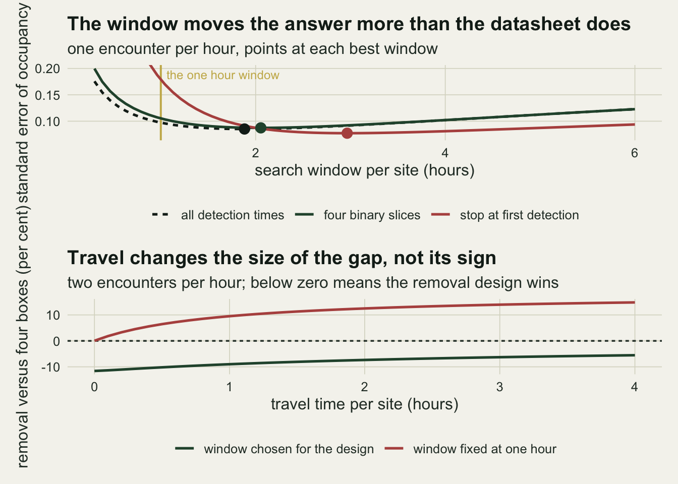
At two encounters per hour and a one hour window, half an hour of travel per site puts the removal design 6.5 per cent behind the four box datasheet and two hours puts it 12.5 per cent behind, which is the conclusion a fixed window forces. Let each design choose its window and the same travel leaves the removal design 10.2 and 7.4 per cent ahead: travel shrinks the advantage without reversing it anywhere in the range measured. What travel does instead is lengthen both windows: at this rate and no travel the best windows are 1.03 and 1.48 hours, and two hours of driving stretches them to 1.52 and 1.92, which is the familiar advice to stay longer at a site that was expensive to reach, arrived at from information rather than from habit. MacKenzie and Royle 2005 make the same point about visits: the comparison has to be made on effort, and each design has to be free to spend that effort its own way.
The recording result survives the change of window in a weaker form. At their own best windows the four box design is 2.5 per cent behind the full record, rather than the 8.3 per cent it was behind at a fixed hour: a longer window recovers part of what the coarse datasheet threw away. The cost of binarising is real, and it is second order next to the length of the visit.
The asymptotic error is not the error you will get
Everything above is Fisher information, which describes the estimator in a sample large enough for the log likelihood to be quadratic near its maximum. A hundred sites at half occupancy is not obviously that sample. Efron and Hinkley 1978 set out why the expected information can be a poor description of a particular fit, so the asymptotics need checking against simulation.
The likelihood makes that check cheap. In every design here, holding the detection parameter fixed, the occupancy that maximises the likelihood is the number of sites with a detection divided by the number of sites at which a detection would be expected if every site were occupied, clipped at one. So occupancy profiles out exactly and what remains is a one dimensional maximisation on a bracket. A general purpose optimiser on the two dimensional logit scale is the wrong tool: the boundary maximum sits at plus infinity in that parameterisation, a quasi-Newton search stops well short of it, and what it reports is a converged fit that is not one.
n_rep <- 20000; n_fits <- 4 * n_rep
sim_full <- function(n_site, psi, lam) rpois(n_site, lam * rbinom(n_site, 1, psi))
sim_slice <- function(n_site, psi, lam, kk)
  rbinom(n_site, kk, rbinom(n_site, 1, psi) * (1 - exp(-lam / kk)))
sim_stop <- function(n_site, psi, lam, ww) {
  wait <- rexp(n_site, lam); found <- rbinom(n_site, 1, psi) == 1 & wait <= ww
  list(found = found, when = wait[found], n = n_site, ww = ww)
}

psi_hat <- function(n_det, n_site, p_det) min(1, n_det / (n_site * p_det))
n_bad <- 0L                                  # counts fits the bracket and grid check rejects
fit_psi <- function(n_det, n_site, p_det, seen, lo, hi) {
  prof <- function(th) {
    ps <- psi_hat(n_det, n_site, p_det(th))
    n_det * log(ps) + seen(th) + (n_site - n_det) * log(ps * (1 - p_det(th)) + 1 - ps)
  }
  op <- optimize(prof, c(lo, hi), maximum = TRUE, tol = 1e-9)
  ok <- op$maximum > lo && op$maximum < hi &&
    op$objective >= max(vapply(seq(lo, hi, length.out = 12), prof, 0)) - 1e-8
  n_bad <<- n_bad + !ok
  psi_hat(n_det, n_site, p_det(op$maximum))
}
fit_stop <- function(obs) fit_psi(sum(obs$found), obs$n, function(a) 1 - exp(-a * obs$ww),
  function(a) sum(obs$found) * log(a) - a * sum(obs$when), 1e-6, 50)

set.seed(4021)
mc_full <- replicate(n_rep, {
  cnt <- sim_full(budget, psi0, lam_lo); pos <- cnt[cnt > 0]
  fit_psi(length(pos), budget, function(a) 1 - exp(-a),
          function(a) sum(dpois(pos, a, log = TRUE)), 1e-6, 50) })
mc_slice <- replicate(n_rep, {
  dd <- sim_slice(budget, psi0, lam_lo, k_std); pos <- dd[dd > 0]
  fit_psi(length(pos), budget, function(a) 1 - (1 - a)^k_std,
          function(a) sum(pos * log(a) + (k_std - pos) * log1p(-a)), 1e-9, 1 - 1e-9) })
mc_stop <- replicate(n_rep, fit_stop(sim_stop(n_lo_use, psi0, lam_lo, 1)))
n_wide <- as.integer(floor(budget / cost_stop_w(lam_lo, w_stop[1])))
mc_wide <- replicate(n_rep, fit_stop(sim_stop(n_wide, psi0, lam_lo, w_stop[1])))

se_stop_mc <- se_psi(info_stop(psi0, lam_lo), n_lo_use)
emp_full <- sd(mc_full); emp_slice <- sd(mc_slice); emp_stop <- sd(mc_stop)
ratio_full <- emp_full / se_full_lo; ratio_slice <- emp_slice / se_k4_lo
ratio_stop <- emp_stop / se_stop_mc; set.seed(88)
pile_stop <- 100 * mean(mc_stop >= 1); bias_stop <- mean(mc_stop) - psi0
pile_wide <- 100 * mean(mc_wide >= 1); bias_wide <- mean(mc_wide) - psi0
boot_sd <- sd(replicate(400, sd(sample(mc_stop, replace = TRUE))))
c(bad = n_bad, r_full = ratio_full, r_slice = ratio_slice, r_stop = ratio_stop)
bad r_full r_slice r_stop
0.000000 1.109583 1.162837 1.231835 Across 20000 simulated surveys at a rate of 1 per hour, the realised standard deviation of the occupancy estimate is 0.1079 for the full record against an asymptotic 0.0973, 0.1224 for four boxes against 0.1053, and 0.2208 for the removal design against 0.1792 on the 122 whole sites the budget buys. The information calculation understates the spread by a factor of 1.11, 1.16 and 1.23, so an interval built from it at this sample size is too narrow, and the understatement grows in step with how weak the design is. None of the 80000 fits failed the bracket and grid check, which is the thing to look at rather than the fact that a fit returned.
The removal design at a one hour window also fails in a specific way rather than simply being noisy. In 14.0 per cent of the surveys the estimate is exactly one, the upper boundary, and the mean estimate sits 0.081 above the truth. A standard error quoted for a run like that describes nothing. That pathology belongs to the window and not to the design: run the same design at its own best window of 2.97 hours on the 51 sites that budget buys, and the boundary rate falls to 0.1 per cent with a bias of 0.012.
mc_lab <- c("all detection times, one hour", "four binary slices, one hour",
            "stop at first detection, one hour", "stop at first detection, best window")  # panels
mc_dat <- data.frame(est = c(mc_full, mc_slice, mc_stop, mc_wide),
  design = factor(rep(mc_lab, each = n_rep), levels = mc_lab))
ggplot(mc_dat, aes(est, fill = design)) +
  geom_histogram(bins = 40, colour = te_paper, linewidth = 0.15) +
  geom_vline(xintercept = psi0, colour = te_body, linetype = "22", linewidth = 0.6) +
  facet_wrap(~ design, ncol = 1, scales = "free_y") +
  scale_fill_manual(values = c(te_ink, te_forest, te_rust, te_gold), guide = "none") +
  scale_x_continuous(breaks = seq(0, 1, 0.2)) +
  labs(x = "estimated occupancy", y = "surveys",
       title = "What the asymptotic standard error is describing",
       subtitle = "dashed line: true occupancy") +
  theme_datasheet() +
  theme(strip.text = element_text(colour = te_ink, hjust = 0))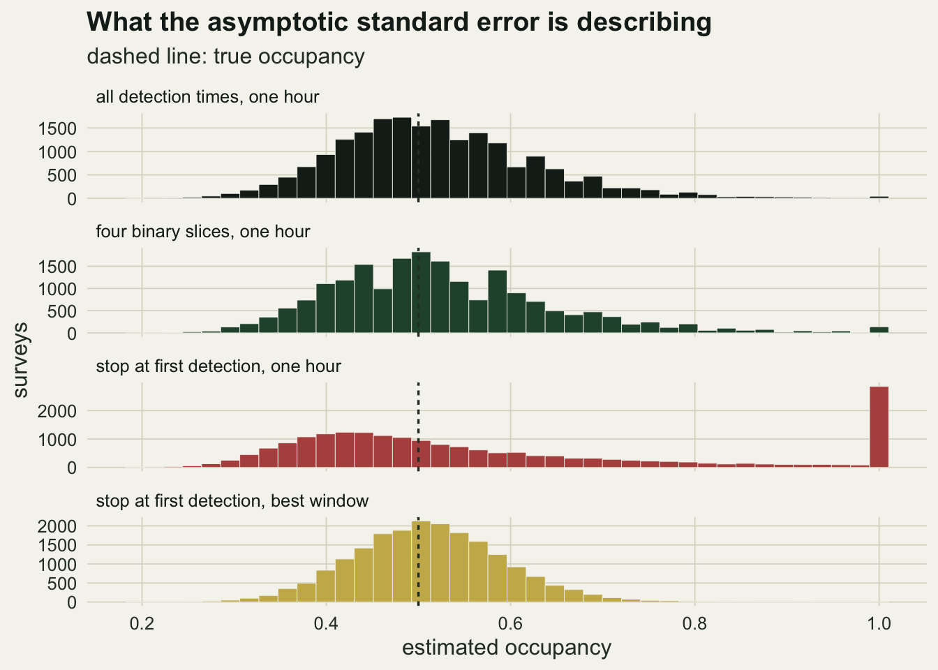
What to report
Give the recording scheme and the search window, not just the number of visits. A survey of four fifteen minute slices within one hour and a survey of four visits on four separate mornings produce the same data matrix and cost entirely different amounts, and only the second is a repeat visit design in the sense the occupancy literature usually means. A comparison of two designs at a window somebody else chose is mostly a comparison of that window.
State the encounter rate the design was planned around and where it came from. Everything here turns on it, and the window most of all, since the best window is the one that puts the expected number of encounters at an occupied site into a narrow range whatever the rate is. A pilot that gives a rough rate is worth more than a finer datasheet, and it is the input that setting a window needs.
Report the cost model explicitly, in the units the budget is actually held in, with travel and setup separated from search: a design comparison quoted in search hours only is a comparison of a quantity nobody pays. If the estimate comes from a small survey, do not quote an asymptotic interval without checking it. Simulating from the fitted values a few thousand times and taking the spread of the refits costs minutes, and it will also show how often the fit runs to the boundary. An occupancy of one with a standard error attached is a report of a failed fit, not a result.
Honest limits
The encounter rate is constant within the window, which no real survey is. A point count starts with the surveyor arriving and settling, birds respond to that disturbance, and detectability changes through the morning. Farnsworth et al. 2002 model a removal count with a constant per minute detection probability and a fraction of the population that is harder to detect, and they list detection changing within a count as an assumption their model does not cover, so the correction is not available off the shelf. Letting the rate decline within the hour costs the slices and not the full record, because the exact times factorise into a shape part orthogonal to occupancy and rate, while the slices see only whether each interval held an encounter.
info_slice_decl <- function(psi, lam0, cc, kk, ww) {
  pat <- as.matrix(expand.grid(rep(list(c(0, 1)), kk))); allz <- rowSums(pat) == 0
  edg <- seq(0, ww, length.out = kk + 1)
  logp <- function(par) {
    mu <- if (abs(par[3]) < 1e-9) rep(par[2] * ww / kk, kk) else
      par[2] * (exp(-par[3] * edg[-(kk + 1)]) - exp(-par[3] * edg[-1])) / par[3]
    pp <- 1 - exp(-mu)
    both <- apply(pat, 1, function(y) prod(ifelse(y == 1, pp, 1 - pp)))
    log(ifelse(allz, par[1] * both + (1 - par[1]), par[1] * both))
  }
  par0 <- c(psi, lam0, cc); prb <- exp(logp(par0))
  gr <- sapply(seq_along(par0), function(i) {
    hh <- 1e-5; pu <- par0; pd <- par0; pu[i] <- pu[i] + hh; pd[i] <- pd[i] - hh
    (logp(pu) - logp(pd)) / (2 * hh) })
  t(gr) %*% (prb * gr)
}
gd <- function(tt, cc) cc * exp(-cc * tt) / (-expm1(-cc))
orth <- max(vapply(c(1, 2, 3, 5), function(cc) abs(integrate(function(tt)
  gd(tt, cc) * (log(gd(tt, cc + 1e-5)) - log(gd(tt, cc - 1e-5))) / 2e-5, 0, 1)$value), 0))
decl_grid <- c(0, 1, 2, 3, 5); fold_grid <- exp(decl_grid)
lam_at_start <- function(cc) if (abs(cc) < 1e-9) lam_lo else lam_lo * cc / (-expm1(-cc))
se_shape <- function(cc) sqrt(solve(info_slice_decl(psi0, lam_at_start(cc), cc, k_std, 1))[1, 1] / budget)
shape_loss <- vapply(decl_grid, function(cc) 100 * (se_shape(cc) / se_full_lo - 1), 0)
rise_loss <- 100 * (se_shape(-1) / se_full_lo - 1)
w_decl <- vapply(decl_grid[1:3], function(cc) optimize(function(w)
  sqrt(solve(info_slice_decl(psi0, lam_lo, cc, k_std, w))[1, 1] / (budget / w)),
  c(0.1, 12))$minimum, 0)
round(c(orth = orth, loss = shape_loss[3], window = w_decl[3]), 5)  # 7.4 fold decline
orth loss window
0.00000 11.86417 0.61274 Take the intensity to fall exponentially across the hour, hold the expected number of encounters at one per occupied hour, and estimate the shape along with everything else. The shape score integrates to \(3.5 \times 10^{-12}\) against the density, so it is orthogonal to occupancy and rate and the full record keeps its 0.0973 for every decline. The four box loss against it grows from 8.3 per cent when the rate is flat to 9.2 per cent at a 2.7 fold decline across the hour, 16.4 per cent at 20.1 fold and 30.9 per cent at 148.4 fold. A rate rising by the same factor costs the same 9.2 per cent as a falling one. The 8.3 per cent headline is therefore a lower bound on what binarising costs, and the exact times are worth more in the field than in this calculation, not less.
That cuts against the window advice, which is derived under a constant rate. A window of 2.05 hours only pays if the species is still calling at the same rate an hour and a half in. Holding the intensity at arrival at one per hour and letting it decline exponentially, the best four box window falls from 2.05 hours when the rate is flat to 1.22 hours at a 2.7 fold decline per hour and 0.61 hours at 7.4 fold. The direction of the window result survives, the size of it does not, and none of it licenses a three hour point count.
The cost model counts field hours and nothing else. Travel is measured above, and setup, permits, equipment and the walk in behave the same way: Field et al. 2005 build a per site overhead, distinct from the per visit cost, into monitoring design for that reason. What no cost term here captures is that one long window at a site and two short ones at two sites are not equally easy to schedule, and that the removal design’s saving cannot be booked in advance, since the field day ends when the birds decide it does.
Occupancy is fixed at psi = 0.5 throughout, and that is not the worst case. Sweeping occupancy with four boxes at the lower rate, the standard error keeps rising with psi across the whole sweep: at 0.95, its top end, it reaches 0.1296 against 0.1053 at a half, because a species present almost everywhere leaves too few empty sites to anchor the all blank ones against. Detection is also independent across slices given occupancy and rate, with no false positives and no site to site variation in the rate. Heterogeneous rates across sites bias occupancy downwards under every design here, which is a different problem from the one measured and is not fixed by finer recording.
The Monte Carlo uses 20000 surveys per design. The empirical standard deviation of the removal estimates carries a bootstrap standard error of 0.00095, which is the one to use rather than the normal theory version for a distribution with 14 per cent of its mass on a boundary point. The ratios of realised to asymptotic spread are separated by far more than that, but a difference of half a per cent between two of them would not be.
References
Garrard G E, Bekessy S A, McCarthy M A, Wintle B A 2008 Austral Ecology 33(8):986-998 (10.1111/j.1442-9993.2008.01869.x)
Bornand C N, Kery M, Bueche L, Fischer M 2014 Methods in Ecology and Evolution 5(5):433-442 (10.1111/2041-210X.12171)
Farnsworth G L, Pollock K H, Nichols J D, Simons T R, Hines J E, Sauer J R 2002 The Auk 119(2):414-425 (10.1093/auk/119.2.414)
MacKenzie D I, Royle J A 2005 Journal of Applied Ecology 42(6):1105-1114 (10.1111/j.1365-2664.2005.01098.x)
Efron B, Hinkley D V 1978 Biometrika 65(3):457-483 (10.1093/biomet/65.3.457)
Field S A, Tyre A J, Possingham H P 2005 Journal of Wildlife Management 69(2):473-482 (10.2193/0022-541X(2005)069[0473:OAOMEU]2.0.CO;2)