library(ggplot2)
library(patchwork)

te_paper  <- "#f5f4ee"
te_ink    <- "#16241d"
te_body   <- "#2c3a31"
te_forest <- "#275139"
te_rust   <- "#b5534e"
te_gold   <- "#c9b458"
te_line   <- "#dad9ca"

theme_datasheet <- function() {
  theme_minimal(base_size = 12) +
    theme(plot.background  = element_rect(fill = te_paper, colour = NA),
          panel.background = element_rect(fill = te_paper, colour = NA),
          panel.grid.major = element_line(colour = te_line, linewidth = 0.3),
          panel.grid.minor = element_blank(),
          text             = element_text(colour = te_body),
          plot.title       = element_text(colour = te_ink, face = "bold"),
          plot.subtitle    = element_text(colour = te_body),
          axis.text        = element_text(colour = te_body),
          strip.text       = element_text(colour = te_ink))
}Time-removal point counts and observer arrival
R
abundance
imperfect detection
point counts
birds
simulation
ecology tutorial
Birds that fall silent as the observer arrives push a time-removal abundance estimate high, most for rare singers. The bias and a settling period in R.
A surveyor walks the last fifty metres to a point in a spruce stand, stops, starts a stopwatch and writes down every bird as it is first heard, minute by minute, for ten minutes. The wren that was singing from the brash pile as she came up the ride has gone quiet. It starts again in the third minute and goes on the sheet as a third-minute bird. Nothing in the data says that it was singing before she arrived, and nothing in the model that will turn those minute-by-minute first detections into a density says so either.
That model is standard. Farnsworth and colleagues (2002) treated the intervals of a point count as removal passes: a bird is removed from the pool of undetected birds the first time it is heard, and the rate at which new birds stop turning up estimates how many were never heard at all. Solymos and colleagues (2013) wrote the same idea in continuous time as a singing rate, the availability half of the QPAD approach they built to calibrate boreal point counts compiled across many studies. In its simplest form the rate is constant within the count. What a detection time is worth names the problem in its closing limits, “A point count starts with the surveyor arriving and settling, birds respond to that disturbance”, notes that Farnsworth and colleagues list a detection rate that changes within the count as an assumption their model does not cover, and leaves it there, because its subject is occupancy. Removal and depletion sampling in R fits Zippin’s discrete-pass removal model by hand; the time-removal model is its continuous-time cousin.
The mechanism here is not new either. Removal estimates when catchability falls shows an electrofishing removal estimate running low when catchability falls from pass to pass. At a point count the observer’s arrival makes the rate rise instead, the estimate runs high, the size of the error is set by how often the species sings, and the obvious repair, starting the stopwatch later, pays only up to a break-even departure rate, and that rate depends on the same singing rate, on how strongly the birds react and on when the disturbed birds leave. Disturbed animals in repeated counts has a removal model broken by the survey as well; there it reads the slow decline of repeated counts as a large population barely dented.
The field evidence does not all point this way. Solymos and colleagues (2018) fitted time-removal models to 152 boreal species and found that finite mixture models, which allow an excess of early detections from a group of frequent singers heard almost at once, fitted better than the constant-rate model. Lee and Marsden (2008), working with distance counts of Philippine forest birds, found density estimates for some groups more than twice as high without a settling period as with one, and read that as birds moving away from the recorder. A rate that rises after arrival and a rate that falls from an early excess or from departures are two opposed within-count patterns, and this post treats song suppression as one of them, not as the pattern. What it measures is how the error depends on the singing rate, whether a calibrated fit test sees it, which way the first minute leans, and what a settling period buys inside a fixed ten-minute budget once birds are allowed to leave while the observer waits.
A bird that sings late
Every bird present at the point when the observer arrives gives cues at a rate phi0 (1 - a exp(-t / tau)) per minute, t minutes after arrival. With a = 0 the rate is constant; with a = 0.9 it starts at a tenth of its undisturbed value and recovers with a time constant tau of 1.5 minutes. The first cue heard after the stopwatch starts is the bird’s first detection. Integrating the rate gives the cumulative hazard phi0 (t - a tau (1 - exp(-t / tau))): after a few multiples of tau the bird behaves as if the clock had started a tau minutes late. Every bird that gives a cue is heard, so detection given availability is one, and the only thing being estimated is availability.
The constant-rate model fitted to the binned first detections is the one of Solymos and colleagues (2013) without covariates. Conditional on the n birds detected in a count of length L, the bins are multinomial with probabilities proportional to exp(-phi t_(j-1)) - exp(-phi t_j), phi is found by maximum likelihood, and the abundance estimate is n divided by 1 - exp(-phi L). The fit test is the likelihood ratio against the saturated multinomial, on (number of bins - 2) degrees of freedom. The design has 300 points with a Poisson mean of two birds each; since the model has no point-level covariates, the counts of all points pool into one multinomial, so each simulated survey is one multinomial draw from a Poisson total. All design constants and grids below were fixed before any simulation ran; the suppression values a and tau and the departure rates later on are a grid, not field estimates.
tau_main  <- 1.5
n_points  <- 300
lam_point <- 2
step_min  <- 0.001
e3  <- c(0, 3, 5, 10)
e10 <- 0:10

cue_H <- function(t, phi0, a, tau) phi0 * (t - a * tau * (1 - exp(-t / tau)))

# bin probabilities for the first cue heard in [s, s + L], plus "never heard";
# d = departure hazard per minute until minute dep_end after arrival,
# f = share flushed at arrival, 1 - mix_c = share that sings at once
cell_probs <- function(phi0, a, tau = tau_main, s = 0, edges = e10,
                       d = 0, dep_end = 0, f = 0, mix_c = 1) {
  tt <- seq(0, s + max(edges), by = step_min)
  hz <- phi0 * (1 - a * exp(-tt / tau))
  Hs <- cue_H(tt, phi0, a, tau) - cue_H(s, phi0, a, tau)
  Dt <- d * pmin(tt, dep_end)
  dens <- ifelse(tt >= s - 1e-9, hz * exp(-Hs - Dt), 0)
  cdf <- c(0, cumsum((dens[-1] + dens[-length(dens)]) / 2 * step_min))
  at <- round((s + edges) / step_min) + 1
  pb <- mix_c * diff(cdf[at])
  pb[1] <- pb[1] + (1 - mix_c) * exp(-d * min(s, dep_end))
  pb <- (1 - f) * pb
  c(pb, 1 - sum(pb))
}

sat_nll <- function(counts) {
  n <- sum(counts)
  -sum(ifelse(counts > 0, counts * log(counts / n), 0))
}

fit_const <- function(counts, edges) {
  n <- sum(counts); len <- max(edges)
  nll <- function(lphi) {
    phi <- exp(lphi)
    -sum(counts * log(diff(-exp(-phi * edges)) / (1 - exp(-phi * len))))
  }
  o <- optimize(nll, c(-8, 4))
  phi <- exp(o$minimum)
  c(phi = phi, n_hat = n / (1 - exp(-phi * len)),
    lr = 2 * (o$objective - sat_nll(counts)), runaway = o$minimum < -7.9)
}

limit_of <- function(pr, edges, fitter = fit_const) {
  big <- 1e6
  fitter(pr[-length(pr)] * big, edges)[["n_hat"]] / big
}

draw_counts <- function(pr, n_draw) {
  n_tot <- rpois(n_draw, n_points * lam_point)
  cnt <- vapply(n_tot, function(nn) as.vector(rmultinom(1, nn, pr)), numeric(length(pr)))
  list(n_tot = n_tot, counts = t(cnt[-length(pr), , drop = FALSE]))
}
Before any sampling noise, the estimator’s destination can be computed from expected bin shares: feed the constant-rate fit the expected counts of a very large survey and read off N-hat / N. That limit is one call to optimize, not a closed form, but it is not a sampling result either, and it is what every simulated median below is heading towards.
phi_show <- 0.15
a_show   <- 0.9
p_true_show <- 1 - exp(-cue_H(10, phi_show, a_show, tau_main))
lag_show    <- a_show * tau_main * (1 - exp(-10 / tau_main))
pr_show     <- cell_probs(phi_show, a_show, edges = e3)
fit_show    <- fit_const(pr_show[1:3] * 1e6, e3)
p_hat_show  <- 1 - exp(-fit_show[["phi"]] * 10)
For a bird singing 0.15 times a minute when undisturbed, with a = 0.9, the chance of being heard at all in ten minutes is 0.727, and by the end of the count the clock is effectively 1.35 minutes late. The constant-rate model fitted to the expected shares in bins of 0 to 3, 3 to 5 and 5 to 10 minutes reads the stretched detection times as a slow singer and puts the chance of being heard at 0.412. The estimate is n divided by that, so it converges to 1.765 times the truth.
The singing rate sets the error
phi_grid <- c(0.10, 0.15, 0.25, 0.30, 0.60, 1.0)
a_grid   <- c(0, 0.5, 0.9)
lim_tab <- expand.grid(phi0 = phi_grid, a = a_grid)
lim_tab$lim3  <- mapply(function(p, a) limit_of(cell_probs(p, a, edges = e3), e3),
                        lim_tab$phi0, lim_tab$a)
lim_tab$lim10 <- mapply(function(p, a) limit_of(cell_probs(p, a), e10),
                        lim_tab$phi0, lim_tab$a)
lim_at <- function(p, a, col = "lim3") lim_tab[lim_tab$phi0 == p & lim_tab$a == a, col]

phi_fine  <- exp(seq(log(0.1), log(1), length.out = 40))
lim_curve <- expand.grid(phi0 = phi_fine, a = c(0.5, 0.9))
lim_curve$lim3 <- mapply(function(p, a) limit_of(cell_probs(p, a, edges = e3), e3),
                         lim_curve$phi0, lim_curve$a)

tau_tab <- expand.grid(phi0 = c(0.15, 0.3), tau = c(0.5, 1.5, 3))
tau_tab$lim3 <- mapply(function(p, tu) limit_of(cell_probs(p, 0.9, tau = tu, edges = e3), e3),
                       tau_tab$phi0, tau_tab$tau)
tau_at <- function(p, tu) tau_tab$lim3[tau_tab$phi0 == p & tau_tab$tau == tu]
n_main <- 1000
set.seed(3271)
main_res <- do.call(rbind, lapply(seq_len(nrow(lim_tab)), function(i) {
pr <- cell_probs(lim_tab$phi0[i], lim_tab$a[i])
dc <- draw_counts(pr, n_main)
c10 <- dc$counts
c3 <- cbind(rowSums(c10[, 1:3]), rowSums(c10[, 4:5]), rowSums(c10[, 6:10]))
f3 <- t(apply(c3, 1, fit_const, edges = e3))
f10 <- t(apply(c10, 1, fit_const, edges = e10))
r3 <- f3[, "n_hat"] / dc$n_tot
data.frame(lim_tab[i, c("phi0", "a")],
med3 = median(r3), q10 = quantile(r3, 0.1), q90 = quantile(r3, 0.9),
run3 = mean(f3[, "runaway"]),
rej3 = mean(pchisq(f3[, "lr"], 1, lower.tail = FALSE) < 0.05),
rej10 = mean(pchisq(f10[, "lr"], 8, lower.tail = FALSE) < 0.05),
det = median(rowSums(c10)))
}))
rownames(main_res) <- NULL
main_at <- function(p, a) main_res[main_res$phi0 == p & main_res$a == a, ]
det_range <- range(main_res$det)The grid crosses six singing rates with three suppression strengths at tau = 1.5 minutes. Each cell holds 1000 simulated surveys, and the median survey detects between 348 and 601 birds depending on the cell, which lies within the range of 200 to 1000 detections that Solymos and colleagues (2018) give as the minimum for reliable time-removal estimates.
With no suppression the estimator is right: the limit is 1.000 at every singing rate. With a = 0.9 the limit is 1.765 for a species singing 0.15 times a minute, 1.134 at 0.30, 1.017 at 0.60 and 1.002 at one cue a minute. With a = 0.5 the same four read 1.194, 1.042, 1.004 and 1.000. A frequent singer is almost sure to be heard some time in ten minutes whatever happens in the first few (chance 0.9998 at one cue a minute and a = 0.9), so n is nearly N and the fitted rate barely matters. A rare singer is heard with chance 0.727 at 0.15 cues a minute, and the estimate divides n by a fitted chance that the stretched depletion curve pulls down. Bins of one minute change the limits little (1.779 and 1.155 for the first two a = 0.9 cells), so the error belongs to the model, not to the coarse bins.
Simulated surveys follow the limits, with the spread that a rare singer brings. At 0.15 cues a minute and a = 0.9 the median is 1.750 with a 10th to 90th percentile range of 1.37 to 2.65, so one survey in ten is too high by more than 165 per cent. At 0.30 the median is 1.135 and the range 1.08 to 1.20. At the rarest singer in the grid, 0.10 cues a minute, the limit is 4.76 and 26 per cent of the a = 0.9 surveys run away: the three bin counts do not decline, the fitted rate goes to its lower bound and the estimate to infinity. That cell is a failure rate, not a number.
bias_pts <- main_res
bias_pts$a_lab <- factor(paste("a =", bias_pts$a))
lim_lines <- rbind(data.frame(phi0 = phi_fine, a = 0, lim3 = 1), lim_curve)
lim_lines$a_lab <- factor(paste("a =", lim_lines$a))
ggplot(bias_pts, aes(phi0, med3, colour = a_lab)) +
  geom_hline(yintercept = 1, colour = te_body, linewidth = 0.4) +
  geom_line(data = lim_lines, aes(y = lim3), linewidth = 0.8) +
  geom_errorbar(aes(ymin = q10, ymax = q90), width = 0.03, linewidth = 0.5) +
  geom_point(size = 2.4) +
  scale_colour_manual(values = c(te_forest, te_gold, te_rust), name = "suppression") +
  scale_x_log10(breaks = phi_grid) +
  scale_y_log10(breaks = c(0.9, 1, 1.25, 1.5, 2, 3)) +
  coord_cartesian(ylim = c(0.85, 3.2)) +
  labs(x = "undisturbed singing rate, cues per minute (log scale)",
       y = "N-hat / N (log scale)",
       title = "Rare singers carry the arrival into the estimate",
       subtitle = "lines: deterministic limit; points: median of 1000 surveys") +
  theme_datasheet() +
  theme(legend.position = "bottom")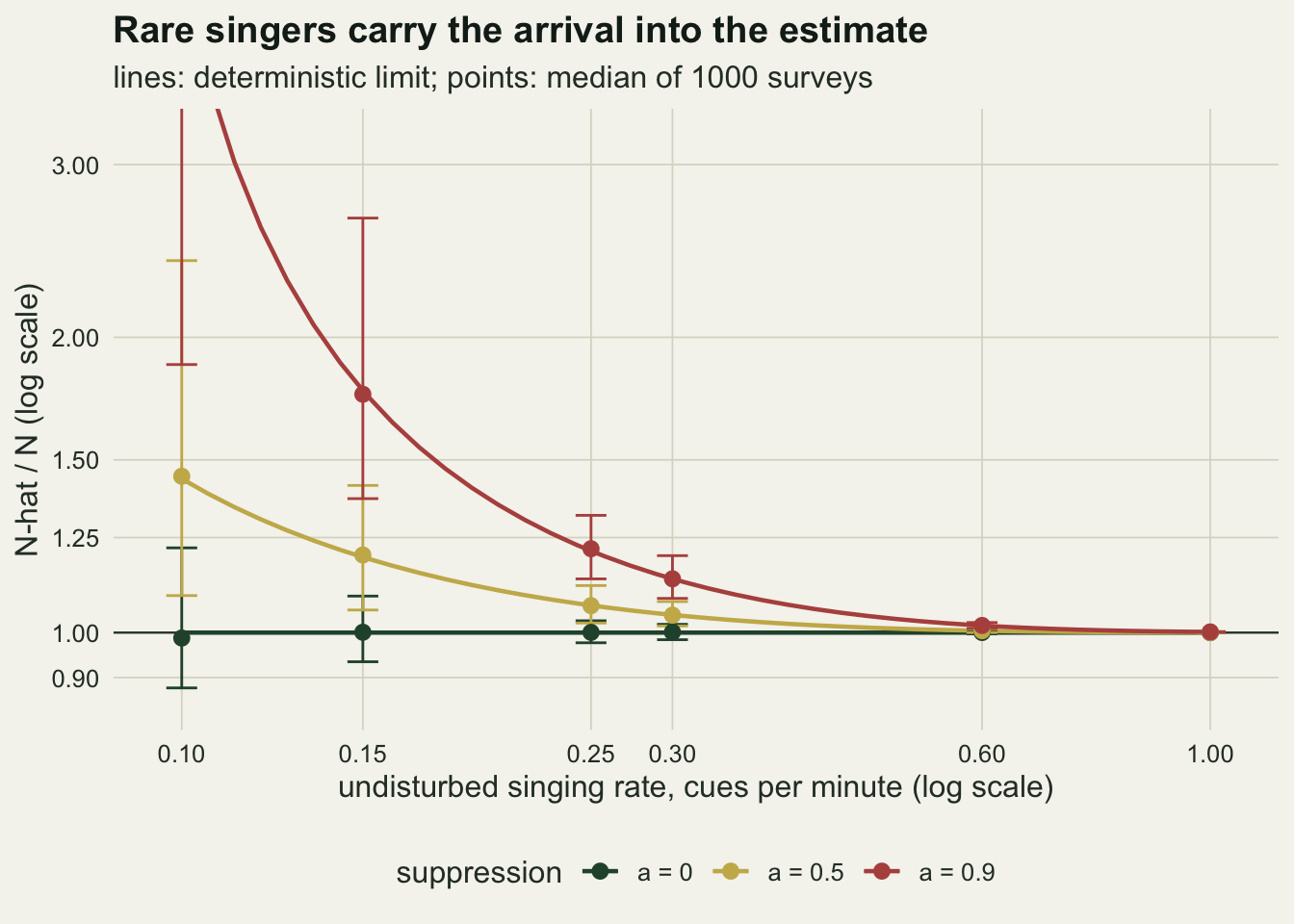
The time constant matters as much as the strength. At a = 0.9 and 0.15 cues a minute the limit is 1.107 when song recovers with tau = 0.5 minutes and 1.765 at 1.5 minutes; at 3 minutes the fit to the expected shares runs away to the edge of the search range. For 0.30 cues a minute the three values are 1.024, 1.134 and 1.504.
flush_f <- 0.2
flush_tab <- expand.grid(phi0 = c(0.15, 0.3, 0.6), a = c(0, 0.9))
flush_tab$lim3 <- mapply(function(p, a) limit_of(cell_probs(p, a, edges = e3, f = flush_f), e3),
                         flush_tab$phi0, flush_tab$a)
flush_gap <- max(abs(flush_tab$lim3 / mapply(lim_at, flush_tab$phi0, flush_tab$a) -
                       (1 - flush_f)))
flush_at <- function(p, a) flush_tab$lim3[flush_tab$phi0 == p & flush_tab$a == a]
set.seed(3272)
n_flush <- 400
flush_sim <- do.call(rbind, lapply(seq_len(nrow(flush_tab)), function(i) {
  pr <- cell_probs(flush_tab$phi0[i], flush_tab$a[i], edges = e3, f = flush_f)
  dc <- draw_counts(pr, n_flush)
  f3 <- t(apply(dc$counts, 1, fit_const, edges = e3))
  data.frame(flush_tab[i, c("phi0", "a")], med = median(f3[, "n_hat"] / dc$n_tot),
             rej3 = mean(pchisq(f3[, "lr"], 1, lower.tail = FALSE) < 0.05))
}))
flush_sim_at <- function(p, a) flush_sim[flush_sim$phi0 == p & flush_sim$a == a, ]
Birds flushed by the observer’s approach are the other arrival effect, and they need no simulation. If a share f leaves before the stopwatch starts and the rest behave as before, every expected bin count is multiplied by 1 - f while the shape of the first-detection times, and so the fitted rate, is unchanged; the estimate is multiplied by exactly 1 - f. On the expected shares the ratio of the flushed to the unflushed limit differs from 0.8 by at most \(3.6 \times 10^{-12}\), and the median of 400 simulated surveys at f = 0.2 and no suppression is 0.801. With suppression the two factors multiply: 1.134 times 0.8 is the 0.908 of a singer at 0.30 cues a minute who loses a fifth of its birds on arrival. That an estimate near one can come out of two errors is arithmetic, and it is not a clean estimate: in that cell the fit test rejects in 0.800 of surveys (against 0.033 to 0.060 with flushing and no suppression), because the suppression is still in the shape.
The fit test, calibrated
A fit test that rejects in more than five per cent of surveys under suppression proves nothing on its own. Removal estimates when catchability falls puts the fair question in its calibration section: does the test reject more often than it does when the model is right, with the same bins? Every rejection share below is therefore printed beside the a = 0 share of the same bin scheme, from the same 1000 surveys per cell as the bias figure, each also cut into one-minute bins. The three-bin test has one degree of freedom; the one-minute test has eight.
mcse_05  <- sqrt(0.05 * 0.95 / n_main)
rej0_3   <- range(main_res$rej3[main_res$a == 0])
rej0_10  <- range(main_res$rej10[main_res$a == 0])
rej9_3   <- range(main_res$rej3[main_res$a == 0.9 & main_res$phi0 >= 0.15])
rej9_10  <- range(main_res$rej10[main_res$a == 0.9 & main_res$phi0 >= 0.15])
With no suppression the three-bin test rejects in 0.045 to 0.061 of surveys across the six singing rates and the one-minute test in 0.014 to 0.060 (the Monte Carlo standard error near 0.05 is 0.007; the lowest one-minute share, at one cue a minute, comes from late bins with almost nothing expected in them). The chi-square reference is therefore close enough to calibrated for this comparison. At a = 0.9 the test sees the suppression: from 0.15 cues a minute upwards the three-bin test rejects in 0.621 to 0.933 of surveys and the one-minute test in 0.962 to 1.000.
The awkward part is where it sees it. At a = 0.5 the one-minute test rejects in 0.329 of surveys for a singer at 0.15 cues a minute, whose one-minute estimate is 20 per cent high, and in 0.810 for a singer at 0.60, whose estimate is 0.6 per cent high. A frequent singer puts hundreds of detections into the first minutes, where the suppression bends the curve, so the shape is measured sharply and the test rejects a model whose abundance estimate is nearly right. A rare singer spreads its detections thinly over the whole count, the bend is measured poorly, and the test is weakest exactly where the estimate is worst. With three bins the contrast is flatter and every share is lower: 0.214 and 0.328 for the same two cells.
gof_long <- rbind(
  data.frame(main_res[, c("phi0", "a")], rej = main_res$rej3, bins = "three bins (0-3-5-10 min)"),
  data.frame(main_res[, c("phi0", "a")], rej = main_res$rej10, bins = "ten one-minute bins"))
gof_long$bins  <- factor(gof_long$bins, levels = c("three bins (0-3-5-10 min)", "ten one-minute bins"))
gof_long$a_lab <- factor(paste("a =", gof_long$a))
gof_long$se    <- sqrt(gof_long$rej * (1 - gof_long$rej) / n_main)
ggplot(gof_long, aes(phi0, rej, colour = a_lab)) +
  geom_hline(yintercept = 0.05, linetype = "dashed", colour = te_body, linewidth = 0.4) +
  geom_errorbar(aes(ymin = pmax(0, rej - 2 * se), ymax = pmin(1, rej + 2 * se)),
                width = 0.03, linewidth = 0.5) +
  geom_line(linewidth = 0.8) +
  geom_point(size = 2) +
  facet_wrap(~ bins) +
  scale_colour_manual(values = c(te_forest, te_gold, te_rust), name = "suppression") +
  scale_x_log10(breaks = c(0.1, 0.3, 1)) +
  scale_y_continuous(limits = c(0, 1)) +
  labs(x = "undisturbed singing rate, cues per minute (log scale)",
       y = "share of surveys rejected",
       title = "The test sees suppression where it matters least",
       subtitle = "dashed: 0.05") +
  theme_datasheet() +
  theme(legend.position = "bottom", panel.spacing = unit(1.4, "lines"))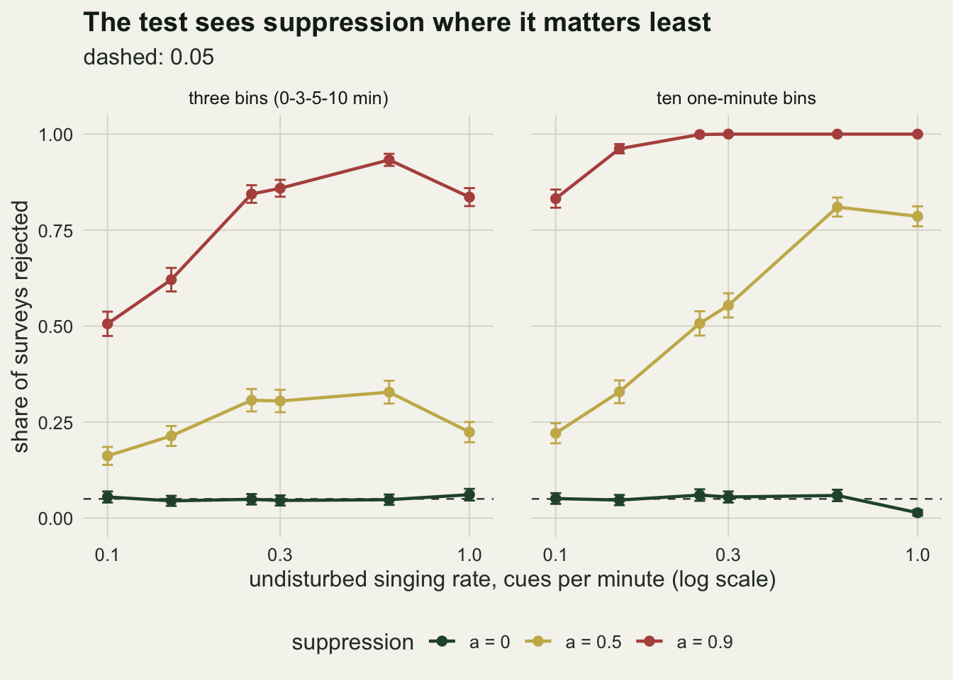
Which way the first minute leans
A rejected fit says the rate was not constant; it does not say which way it moved. The residuals do. The figure below fits the constant-rate model to the expected one-minute shares of four truths at 0.3 cues a minute and plots observed over expected by minute: song suppression at two strengths, a mixture in which 30 per cent of birds sing the moment the observer arrives and the rest at the constant rate (the early excess of the finite mixture models), and no suppression but departures at 0.1 per minute during the first three minutes after arrival, in which a bird that leaves before it has been heard is lost.
fit_mix <- function(counts, edges) {
  n <- sum(counts); len <- max(edges)
  nll <- function(th) {
    phi <- exp(th[1]); cc <- plogis(th[2])
    cdf <- 1 - cc * exp(-phi * edges); cdf[1] <- 0
    pr <- diff(cdf) / cdf[length(cdf)]
    if (any(!is.finite(pr)) || any(pr <= 0)) return(1e10)
    -sum(counts * log(pr))
  }
  starts <- list(c(log(0.2), 2), c(log(0.2), 0), c(log(0.5), -1))
  fits <- lapply(starts, function(st) optim(st, nll))
  best <- fits[[which.min(vapply(fits, function(o) o$value, 0))]]
  phi <- exp(best$par[1]); cc <- plogis(best$par[2])
  c(n_hat = n / (1 - cc * exp(-phi * len)), c_hat = cc,
    lr = 2 * (best$value - sat_nll(counts)))
}

fit_shift <- function(counts, edges, max_shift = 3) {
  n <- sum(counts); len <- max(edges)
  nll <- function(th) {
    phi <- exp(th[1]); shift <- max_shift * plogis(th[2])
    cdf <- 1 - exp(-phi * pmax(0, edges - shift))
    pr <- pmax(diff(cdf) / cdf[length(cdf)], 1e-300)
    -sum(counts * log(pr))
  }
  starts <- list(c(log(0.2), -3), c(log(0.2), -1), c(log(0.5), 0))
  fits <- lapply(starts, function(st) optim(st, nll))
  best <- fits[[which.min(vapply(fits, function(o) o$value, 0))]]
  phi <- exp(best$par[1]); shift <- max_shift * plogis(best$par[2])
  c(n_hat = n / (1 - exp(-phi * (len - shift))), shift = shift,
    lr = 2 * (best$value - sat_nll(counts)))
}

oe_by_minute <- function(pr) {
  ex <- pr[-length(pr)] * 1e6
  fc <- fit_const(ex, e10)
  fitted <- sum(ex) * diff(-exp(-fc[["phi"]] * e10)) / (1 - exp(-fc[["phi"]] * 10))
  ex / fitted
}
phi_shape <- 0.3
excess_c  <- 0.7
dep_show  <- 0.1
shape_labs <- c("song suppressed, a = 0.5", "song suppressed, a = 0.9",
                "30 per cent sing at once", "departures in minutes 0 to 3")
shape_df <- rbind(
  data.frame(minute = 1:10, oe = oe_by_minute(cell_probs(phi_shape, 0.5)), truth = shape_labs[1]),
  data.frame(minute = 1:10, oe = oe_by_minute(cell_probs(phi_shape, 0.9)), truth = shape_labs[2]),
  data.frame(minute = 1:10, oe = oe_by_minute(cell_probs(phi_shape, 0, mix_c = excess_c)),
             truth = shape_labs[3]),
  data.frame(minute = 1:10, oe = oe_by_minute(cell_probs(phi_shape, 0, d = dep_show, dep_end = 3)),
             truth = shape_labs[4]))
shape_df$truth <- factor(shape_df$truth, levels = shape_labs)
oe_at <- function(k, m = 1) shape_df$oe[shape_df$truth == shape_labs[k] & shape_df$minute == m]
lim_excess <- limit_of(cell_probs(phi_shape, 0, mix_c = excess_c), e10)
lim_dep    <- limit_of(cell_probs(phi_shape, 0, d = dep_show, dep_end = 3), e10)
Suppression leaves the first minute short: observed over expected is 0.822 at a = 0.5 and 0.568 at a = 0.9, with the missing birds turning up in minutes two to six. The early-excess mixture leans the other way, 1.338 in the first minute, and its constant-rate estimate runs low, at 0.975 in the limit. Departures lean the same way as the excess but far more weakly, 1.054 in the first minute, while the estimate falls to 0.816: birds that leave unheard take their share of the total with them and leave the shape of the curve nearly intact. The sign of the first-minute residual is the cheapest way to tell which of the two opposed patterns a survey is showing, which is the question a methodologist would put to any large compilation of point counts; this post has no field data to answer it.
ggplot(shape_df, aes(minute, oe, colour = truth)) +
  geom_hline(yintercept = 1, colour = te_body, linewidth = 0.4) +
  geom_line(linewidth = 0.8) +
  geom_point(size = 2) +
  scale_colour_manual(values = c(te_gold, te_rust, te_forest, te_ink), name = NULL) +
  scale_x_continuous(breaks = 1:10) +
  labs(x = "minute of the count", y = "observed / expected under constant rate",
       title = "The first minute leans one way or the other",
       subtitle = "expected shares, 0.3 cues per minute") +
  theme_datasheet() +
  theme(legend.position = "bottom") +
  guides(colour = guide_legend(nrow = 2))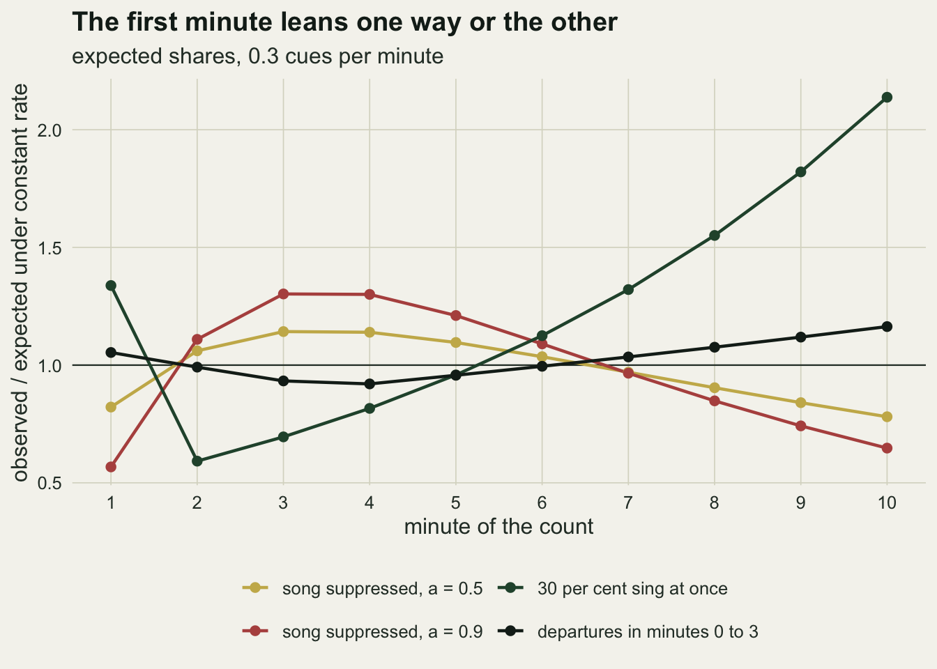
The residual direction also says which extension of the model can help. The finite mixture of Farnsworth and colleagues, written in continuous time as a share 1 - c of birds heard at once and a share c singing at rate phi, can only add birds to the first bin. A delayed start can only take them away. The second model is written here for this post: a constant rate that begins after a shift of up to three minutes, so the chance of being heard by time t is 1 - exp(-phi max(0, t - shift)) and the estimate is n divided by 1 - exp(-phi (10 - shift)). It is not the true suppression curve, and it has one parameter more than the constant model. Both are fitted by maximum likelihood to one-minute bins, 200 surveys per cell.
n_shape <- 200
shape_cells <- rbind(expand.grid(phi0 = c(0.15, 0.3, 0.6), a = a_grid, mix_c = 1),
                     data.frame(phi0 = c(0.15, 0.3), a = 0, mix_c = excess_c))
set.seed(3273)
shape_res <- do.call(rbind, lapply(seq_len(nrow(shape_cells)), function(i) {
  pr <- cell_probs(shape_cells$phi0[i], shape_cells$a[i], mix_c = shape_cells$mix_c[i])
  dc <- draw_counts(pr, n_shape)
  fc <- t(apply(dc$counts, 1, fit_const, edges = e10))
  fs <- t(apply(dc$counts, 1, fit_shift, edges = e10))
  fm <- t(apply(dc$counts, 1, fit_mix, edges = e10))
  rc <- fc[, "n_hat"] / dc$n_tot
  rs <- fs[, "n_hat"] / dc$n_tot
  data.frame(shape_cells[i, ],
             med_c = median(rc), rmse_c = sqrt(mean((rc - 1)^2)),
             med_s = median(rs), rmse_s = sqrt(mean((rs - 1)^2)),
             shift_med = median(fs[, "shift"]), shift_q10 = quantile(fs[, "shift"], 0.1),
             shift_q90 = quantile(fs[, "shift"], 0.9),
             med_m = median(fm[, "n_hat"] / dc$n_tot), c_one = mean(fm[, "c_hat"] > 0.99),
             rej_mix   = mean(pchisq(fc[, "lr"] - fm[, "lr"], 1, lower.tail = FALSE) < 0.05),
             rej_shift = mean(pchisq(fc[, "lr"] - fs[, "lr"], 1, lower.tail = FALSE) < 0.05))
}))
rownames(shape_res) <- NULL
sh_at <- function(p, a, mc = 1) shape_res[shape_res$phi0 == p & shape_res$a == a &
                                          shape_res$mix_c == mc, ]
c_one_supp <- min(shape_res$c_one[shape_res$a > 0])
rej_shift_0 <- range(shape_res$rej_shift[shape_res$a == 0 & shape_res$mix_c == 1])
rej_mix_0   <- range(shape_res$rej_mix[shape_res$a == 0 & shape_res$mix_c == 1])
Under suppression the mixture is no help at all: its estimate of c sits on the boundary of one, where it collapses to the constant model, in every survey of every suppressed cell, and its median estimate at 0.15 cues a minute and a = 0.9 is 1.856. On the early-excess truth it recovers the population (median 1.009 at 0.15 cues a minute, against 0.873 for the constant model), and its likelihood-ratio test against the constant model rejects in 1.000 of those surveys (against 0.020 to 0.035 in unsuppressed cells without the early group). The delayed-start model is the mirror image. On the early-excess truth its shift is estimated at zero and it adds nothing; under suppression it takes much of the error away. At 0.15 cues a minute and a = 0.9 its median is 1.229 with a root mean square error of 0.336, against 1.835 and 1.332 for the constant model; at a = 0.5 the medians are 1.086 against 1.201, and at 0.3 cues a minute and a = 0.9 1.054 against 1.156. Without suppression its error is 0.057 against 0.056 at 0.15 cues a minute, so the extra parameter costs little.
Is the shift identifiable from one-minute bins at 300 points? Here, yes, in the sense that the data move it: at 0.15 cues a minute its median is 0.28 minutes at a = 0.5 and 0.57 at a = 0.9, with a 10th to 90th percentile range at a = 0.9 of 0.44 to 0.66, and its test against the constant model rejects in 0.015 to 0.025 of unsuppressed surveys (the test is conservative because a shift of zero lies on the edge of its range, and the same holds for the mixture at c = 1) and in 0.560 of surveys at 0.15 cues a minute and a = 0.5. But the fitted shift is shorter than the late clock of the true process (0.75 and 1.35 minutes), because a gradual recovery is not a sharp start, and that is why the rare-singer estimate is improved rather than repaired.
A settling period, when birds leave
The usual field repair is to wait: stand at the point for s minutes before starting the stopwatch, and count for the rest of a fixed ten-minute visit in one-minute bins. If no bird leaves, waiting skips the minutes in which the rate is lowest, but it also shortens the count. The question is what happens when birds do leave, and here the model has to say when. Two versions are run. In the first, birds leave at d per minute only while the observer waits and stop when the stopwatch starts; this is the version in which waiting is a pure loss of birds. In the second, birds that react to the arrival leave at d per minute during the first three minutes after arrival whatever the stopwatch says, so a count started at once records some of them before they go and a count started after three minutes records none. In both, N is every bird present before the observer arrived. Each cell of four settling times, seven departure rates and four combinations of singing rate and suppression holds 400 surveys; the delayed-start model fitted to a count started at once is run alongside on 200 surveys per cell.
bud_cells <- expand.grid(phi0 = c(0.15, 0.3), a = c(0.5, 0.9))
d_grid <- c(0, 0.025, 0.05, 0.1, 0.15, 0.2, 0.3)
s_grid <- 0:3
v_names <- c("leave only while waiting", "leave in the first 3 minutes")
dep_window <- 3
n_bud <- 400
n_bud_shift <- 200
# in version one a count started at once does not depend on d, so s = 0 is run once
bud_design <- rbind(
  expand.grid(cell = 1:4, s = s_grid, d = d_grid[1], version = v_names[1],
              stringsAsFactors = FALSE),
  expand.grid(cell = 1:4, s = s_grid[-1], d = d_grid[-1], version = v_names[1],
              stringsAsFactors = FALSE),
  expand.grid(cell = 1:4, s = s_grid, d = d_grid[-1], version = v_names[2],
              stringsAsFactors = FALSE))
set.seed(3274)
bud_res <- do.call(rbind, lapply(seq_len(nrow(bud_design)), function(i) {
  bd <- bud_design[i, ]; cl <- bud_cells[bd$cell, ]
  ed <- 0:(10 - bd$s)
  dep_end <- if (bd$version == v_names[1]) bd$s else dep_window
  pr <- cell_probs(cl$phi0, cl$a, s = bd$s, edges = ed, d = bd$d, dep_end = dep_end)
  dc <- draw_counts(pr, n_bud)
  fc <- t(apply(dc$counts, 1, fit_const, edges = ed))
  rc <- fc[, "n_hat"] / dc$n_tot
  data.frame(cl, bd, lim = limit_of(pr, ed), med = median(rc), rmse = sqrt(mean((rc - 1)^2)),
             mae = median(abs(rc - 1)), max = max(rc), runaway = sum(fc[, "runaway"]), copy = FALSE,
             rej = mean(pchisq(fc[, "lr"], length(ed) - 3, lower.tail = FALSE) < 0.05))
}))
zero_v1 <- bud_res[bud_res$version == v_names[1] & bud_res$s == 0, ]
bud_res <- rbind(bud_res,
                 do.call(rbind, lapply(d_grid[-1], function(dd) transform(zero_v1, d = dd, copy = TRUE))),
                 transform(bud_res[bud_res$d == 0, ], version = v_names[2], copy = TRUE))
rownames(bud_res) <- NULL
bud_at <- function(p, a, s, d, v = v_names[1]) {
  bud_res[bud_res$phi0 == p & bud_res$a == a & bud_res$s == s &
            abs(bud_res$d - d) < 1e-9 & bud_res$version == v, ]
}

set.seed(3275)
shift_bud <- do.call(rbind, lapply(seq_len(4 * length(d_grid)), function(i) {
  cl <- bud_cells[(i - 1) %% 4 + 1, ]; dd <- d_grid[(i - 1) %/% 4 + 1]
  pr <- cell_probs(cl$phi0, cl$a, d = dd, dep_end = dep_window)
  dc <- draw_counts(pr, n_bud_shift)
  rs <- apply(dc$counts, 1, function(x) fit_shift(x, e10)[["n_hat"]]) / dc$n_tot
  data.frame(cl, d = dd, med = median(rs), rmse = sqrt(mean((rs - 1)^2)))
}))
shift_at <- function(p, a, d) shift_bud[shift_bud$phi0 == p & shift_bud$a == a &
                                          abs(shift_bud$d - d) < 1e-9, ]

# calibration reference for the budget fit tests: no suppression, no departures
set.seed(3276)
calib <- do.call(rbind, lapply(seq_len(8), function(i) {
  pp <- c(0.15, 0.3)[(i - 1) %% 2 + 1]; ss <- s_grid[(i - 1) %/% 2 + 1]
  ed <- 0:(10 - ss)
  dc <- draw_counts(cell_probs(pp, 0, s = ss, edges = ed), n_bud)
  fc <- t(apply(dc$counts, 1, fit_const, edges = ed))
  data.frame(phi0 = pp, s = ss,
             rej = mean(pchisq(fc[, "lr"], length(ed) - 3, lower.tail = FALSE) < 0.05))
}))
calib_range <- range(calib$rej)

# version one: waiting multiplies the limit by exactly exp(-d s)
v1 <- bud_res[bud_res$version == v_names[1] & bud_res$s > 0, ]
v1_base <- mapply(function(p, a, s) bud_at(p, a, s, 0)$lim, v1$phi0, v1$a, v1$s)
v1_gap <- max(abs(v1$lim / v1_base - exp(-v1$d * v1$s)))

# the departure rate at which two minutes of settling stop beating none, as a grid bracket
bracket <- function(p, a, v, metric = "rmse") {
  gap <- sapply(d_grid, function(dd) bud_at(p, a, 2, dd, v)[[metric]] - bud_at(p, a, 0, dd, v)[[metric]])
  k <- which(gap >= 0)[1]
  if (is.na(k)) return(c(max(d_grid), Inf))
  if (k == 1) return(c(0, 0))
  c(d_grid[k - 1], d_grid[k])
}
br_all <- function(metric) lapply(seq_len(8), function(i) {
  cl <- bud_cells[(i - 1) %% 4 + 1, ]; v <- v_names[(i - 1) %/% 4 + 1]
  bracket(cl$phi0, cl$a, v, metric)
})
br     <- br_all("rmse")
br_mae <- br_all("mae")
br_txt <- function(i, brs = br) {
  b <- brs[[i]]
  if (is.infinite(b[2])) return(sprintf("above %.1f", b[1]))
  if (b[2] == 0) return("at zero, since it does not pay even without departures,")
  sprintf("between %.3f and %.3f", b[1], b[2])
}
# the same brackets on the median absolute error, which a rare very large estimate does not move
br_same  <- vapply(seq_len(8), function(i) identical(br[[i]], br_mae[[i]]), logical(1))
br_step1 <- all(vapply(which(!br_same), function(i)
  match(br_mae[[i]][2], d_grid) == match(br[[i]][2], d_grid) - 1, logical(1)))
cell_txt <- function(i) {
  cl <- bud_cells[(i - 1) %% 4 + 1, ]
  sprintf("%g cues a minute and a = %.1f in the %s version", cl$phi0, cl$a,
          c("first", "second")[(i - 1) %/% 4 + 1])
}
mae_txt <- paste(vapply(which(!br_same), function(i)
  sprintf("%s instead of %s for %s", br_txt(i, br_mae), br_txt(i), cell_txt(i)), ""), collapse = "; ")
oe_cancel <- oe_by_minute(cell_probs(0.3, 0.9, d = 0.05, dep_end = dep_window))[1]
run_total <- sum(bud_res$runaway[!bud_res$copy])
run_fits  <- n_bud * sum(!bud_res$copy)
run_cell  <- bud_res[bud_res$runaway > 0 & !bud_res$copy, ][1, ]

# the delayed-start fit against the best and against the two-minute settling time, version two
v2_res  <- bud_res[bud_res$version == v_names[2], ]
v2_best <- aggregate(rmse ~ phi0 + a + d, v2_res, min)
v2_two  <- v2_res[v2_res$s == 2, c("phi0", "a", "d", "rmse")]
sh_cmp  <- merge(merge(v2_best, v2_two, by = c("phi0", "a", "d"), suffixes = c("_best", "_two")),
                 shift_bud[, c("phi0", "a", "d", "rmse")], by = c("phi0", "a", "d"))
sh_ratio  <- range(sh_cmp$rmse / sh_cmp$rmse_best)
sh_beats2 <- sum(sh_cmp$rmse < sh_cmp$rmse_two)
best_s_n  <- length(unique(v2_res$s[v2_res$rmse %in% v2_best$rmse]))
sh_below  <- sum(sh_cmp$rmse < sh_cmp$rmse_best)
sh_near   <- sum(sh_cmp$rmse / sh_cmp$rmse_best < 1.1)
With no departures, two minutes of settling cut the root mean square error of N-hat / N from 1.321 to 0.214 for a singer at 0.15 cues a minute and a = 0.9, and from 0.054 to 0.033 at 0.3 cues a minute and a = 0.5. That is the pilot’s case for waiting, and it assumes that every bird stays. Even then the wait is not free, because it shortens the count: at 0.15 cues a minute and a = 0.5, three minutes of waiting bring the limit from 1.199 to 1.033 yet leave a larger root mean square error than none (0.333 against 0.260), because a seven-minute count of a rare singer can return a very large estimate (the largest of the 400 in that cell is 7.05 times the truth); the median absolute error does fall, from 0.190 to 0.071.
In the first version the departures do nothing but remove birds before the count, exactly like flushing: the limit is multiplied by exp(-d s), which the expected shares confirm to within \(4.5 \times 10^{-12}\). Where two minutes of settling stop beating none follows from that factor and from the spread, and the grid places it between 0.150 and 0.200 per minute for 0.15 cues a minute and a = 0.5, between 0.025 and 0.050 for 0.3 and a = 0.5, above 0.3 for 0.15 and a = 0.9, and between 0.100 and 0.150 for 0.3 and a = 0.9. A frequent singer with mild suppression has little bias to remove, so a departure rate of a few per cent per minute is enough to make the wait a loss; a rare singer under strong suppression starts so far out that waiting pays across the whole grid.
In the second version the count started at once also sees departures, and they pull its estimate down against the suppression’s upward error. The break-even rates fall to between 0.025 and 0.050, between 0.000 and 0.025, between 0.100 and 0.150 and between 0.025 and 0.050 per minute for the same four cells. This is the cancellation that the flushing paragraph warned about, and it is visible. At 0.3 cues a minute, a = 0.9 and d = 0.05, the count started at once has a limit of 1.000 and an error of 0.039, better than the 0.112 of two minutes’ wait, yet its one-minute fit test rejects in 0.993 of surveys. The two-minute count, whose estimate is 0.890, rejects in 0.070, against 0.037 to 0.065 in the no-suppression, no-departure reference cells of the same bin schemes. Settling trades an error the fit test can see for one it cannot: birds lost before the stopwatch starts leave no mark on the shape of the count.
The delayed-start model on a count started at once is often close to the best settling time and sometimes well behind it. Under the second version its error at 0.15 cues a minute and a = 0.9 is 0.350 without departures, 0.167 at d = 0.05 and 0.150 at d = 0.1, against 0.214, 0.143 and 0.206 for two minutes of settling. Over the 28 combinations of cell and departure rate in that version its error is between 0.88 and 2.05 times that of the best of the four settling times, picked with hindsight for each combination: no more than ten per cent worse than it in 15, below it in 5, and better than a fixed two-minute wait in 23. What it offers is that it needs no choice: the best settling time in that version takes 4 different values across the grid, and picking it requires the departure rate and the suppression that nobody measures. In the first version, where no bird leaves once the stopwatch runs, the count started at once does not depend on d at all, so the delayed-start fit keeps its no-departure error while the estimate of every settling time is multiplied by exp(-d s). One of the 73600 budget fits ran away, in the cell where birds leave in the first 3 minutes, at 0.15 cues a minute, a = 0.9, s = 0 and d = 0.025; it takes that cell’s root mean square error to 9.8, off the top of the figure. Draws that stop short of that bound but still return a very large estimate lift single cells as well: three minutes of settling at d = 0.3 in the first version, for the same singer, has a root mean square error of 1.14 around a limit of 0.433.
bud_plot <- bud_res
bud_plot$series <- paste("settle", bud_plot$s, "min")
shift_zero <- shift_bud[rep(which(shift_bud$d == 0), length(d_grid)), c("phi0", "a", "rmse")]
shift_zero$d <- rep(d_grid, each = 4)
shift_plot <- rbind(
  data.frame(shift_zero[, c("phi0", "a", "d", "rmse")], version = v_names[1]),
  data.frame(shift_bud[, c("phi0", "a", "d", "rmse")], version = v_names[2]))
shift_plot$series <- "start at once, delayed-start fit"
bud_plot <- rbind(bud_plot[, c("phi0", "a", "d", "rmse", "version", "series")], shift_plot)
bud_plot$cell <- factor(sprintf("phi0 %.2f, a = %.1f", bud_plot$phi0, bud_plot$a))
bud_plot$version <- factor(ifelse(bud_plot$version == v_names[1], "only while waiting",
                                   "first 3 minutes"),
                            levels = c("only while waiting", "first 3 minutes"))
bud_plot$series <- factor(bud_plot$series,
                          levels = c(paste("settle", s_grid, "min"), "start at once, delayed-start fit"))
ggplot(bud_plot, aes(d, rmse, colour = series, linetype = series)) +
  geom_line(linewidth = 0.7) +
  geom_point(size = 1.3) +
  facet_grid(version ~ cell) +
  scale_colour_manual(values = c(te_rust, te_gold, te_forest, te_ink, te_body), name = NULL) +
  scale_linetype_manual(values = c("solid", "solid", "solid", "solid", "dashed"), name = NULL) +
  scale_y_log10() +
  coord_cartesian(ylim = c(0.02, 1.5)) +
  scale_x_continuous(breaks = c(0, 0.1, 0.2, 0.3)) +
  labs(x = "departure rate d, per minute", y = "RMSE of N-hat / N (log scale)",
       title = "Whether waiting pays depends on who leaves, and when",
       subtitle = "fixed ten-minute visit, 300 points") +
  theme_datasheet() +
  theme(legend.position = "bottom", panel.spacing = unit(1, "lines"),
        strip.text = element_text(size = 9)) +
  guides(colour = guide_legend(nrow = 2))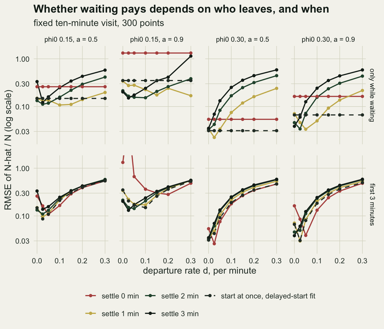
What to report
Record first detections in one-minute bins, not in three or four long intervals. The one-minute bins cost nothing in the field, they give the fit test eight degrees of freedom instead of one, and they are what the first-minute residual and the two model extensions need.
Report the sign of the first-minute residual under the constant-rate fit, by species or species group, along with the fit test. A first minute that is short points to a rate that rises after arrival and an estimate that is too high, unless birds are also leaving early, which pulls the estimate back down without removing the short first minute (at 0.3 cues a minute, a = 0.9 and d = 0.05 in the first three minutes, the first minute holds 0.600 of its expected share while the limit is 1.000); a first minute in excess points to the early-singing group of the finite mixture, or to birds leaving, and an estimate that is too low. A passed fit test is not evidence of a constant rate for a rare singer: at a = 0.5 and 0.15 cues a minute the one-minute test missed the suppression in 0.671 of surveys while the estimate ran 20 per cent high.
If a settling period is used, report its length and count the birds seen or heard leaving during it. The departure rate decides whether the wait helped, and without it the settling period hides its own error from every test in the data.
Treat a constant-rate estimate for a species with a low singing rate as sensitive to how the birds reacted to the observer, in either direction, and check it against the delayed-start and mixture fits before reporting it.
Honest limits
The suppression curve is one exponential recovery with a single a and tau shared by every bird, and the grid of a and tau values is not taken from any species. Real birds differ within a species in how much and for how long they react, and a mixture of reactions would give a residual shape somewhere between the curves shown here. Nothing in the post estimates a or tau for any bird.
The departure model is also a choice. The two versions bracket two ideas of when a disturbed bird leaves, and neither is fitted to data. Lee and Marsden’s factor of two cannot be turned into a departure rate here: in this model suppression alone, with no bird leaving, makes the median estimate from a count started at once 1.6 times the one after two minutes of settling at 0.15 cues a minute and a = 0.9, and the movement they describe changes detection distance rather than removing birds. The break-even rates are grid brackets from 400 surveys per cell, and a root mean square error is sensitive to the rare very large estimate of a rare singer. On the median absolute error, which such an estimate does not move, the brackets agree in 5 of the 8 cells and are one grid step lower in the others: between 0.100 and 0.150 instead of between 0.150 and 0.200 for 0.15 cues a minute and a = 0.5 in the first version; between 0.050 and 0.100 instead of between 0.100 and 0.150 for 0.3 cues a minute and a = 0.9 in the first version; between 0.050 and 0.100 instead of between 0.100 and 0.150 for 0.15 cues a minute and a = 0.9 in the second version.
Detection given availability is one throughout: every cue is heard, at any distance. In a real point count the distance half of QPAD enters too, and a bird that moves away from the observer changes its detection distance rather than vanishing, which is the mechanism Lee and Marsden describe for distance counts. The 300 points pool into one multinomial because there are no point-level covariates; with covariates on the singing rate, as in the Solymos framework, point-level heterogeneity would add a mixture of its own.
The delayed-start model is written for this post as the counterpart of the mixture, and it was checked only on data simulated from the suppression model it is meant to approximate. That it improves the estimate here says that a sharp start approximates a gradual recovery reasonably well, not that it would behave as well on real counts or together with an early-singing group in the same species.
References
Farnsworth GL, Pollock KH, Nichols JD, Simons TR, Hines JE, Sauer JR 2002 The Auk 119(2):414-425 (10.1093/auk/119.2.414)
Solymos P, Matsuoka SM, Bayne EM, Lele SR, Fontaine P, Cumming SG, Stralberg D, Schmiegelow FKA, Song SJ 2013 Methods in Ecology and Evolution 4(11):1047-1058 (10.1111/2041-210X.12106)
Solymos P, Matsuoka SM, Cumming SG, Stralberg D, Fontaine P, Schmiegelow FKA, Song SJ, Bayne EM 2018 The Condor 120(4):765-786 (10.1650/CONDOR-18-32.1)
Lee DC, Marsden SJ 2008 Ibis 150(2):315-325 (10.1111/j.1474-919X.2007.00790.x)