library(ggplot2)
library(patchwork)

te_paper  <- "#f5f4ee"
te_ink    <- "#16241d"
te_body   <- "#2c3a31"
te_forest <- "#275139"
te_rust   <- "#b5534e"
te_gold   <- "#c9b458"
te_line   <- "#dad9ca"

theme_datasheet <- function() {
  theme_minimal(base_size = 12) +
    theme(plot.background  = element_rect(fill = te_paper, colour = NA),
          panel.background = element_rect(fill = te_paper, colour = NA),
          panel.grid.major = element_line(colour = te_line, linewidth = 0.3),
          panel.grid.minor = element_blank(),
          text             = element_text(colour = te_body),
          plot.title       = element_text(colour = te_ink, face = "bold"),
          plot.subtitle    = element_text(colour = te_body),
          axis.text        = element_text(colour = te_body))
}Disturbed animals in repeated counts
R
abundance
imperfect detection
N-mixture
behavioural response
simulation
ecology tutorial
When a counted animal hides on later visits, N-mixture and removal estimates both run high, each failing at one end. A count-only Mb model in R bridges them.
A salamander survey turns the same 150 cover boards four times in a fortnight and writes down how many red-backed salamanders are under each one. The counts fall a little from visit to visit, which is what counts do when some of the animals found on the first morning have moved to a stone or a log that nobody turns. Marsh and Goicochea (2003) tested this with wooden cover boards and found that daily sampling reduced salamander counts substantially, mostly in adults, while weekly sampling did no worse than sampling every three weeks. Handling or exposing an animal changes where it will be on the next visit. Turn a board, flush a bird from a hedge or lift a crayfish out of a riffle and put it back, and the animal that was counted is no longer the animal it was.
Repeated counts of unmarked animals are usually analysed with the binomial N-mixture model of Royle (2004), fitted by hand on this site in N-mixture models for abundance in R. The model assumes that every animal present on a visit has the same chance of being counted, whatever happened on earlier visits. N-mixture reliability and the detection trade-off breaks that assumption with detection heterogeneity drawn afresh for every site and visit, so it is shared by every animal present at that moment and is not caused by the count; Link, Schofield, Barker and Sauer (2018) showed how far small departures of that kind can move an N-mixture estimate. Here the count itself makes a counted animal different, and there are no marks to model it with. With marks this is model Mb, the trap-shy row of Capture heterogeneity: Mt, Mb and Mh in R, where animals that avoid traps after their first capture look like animals that were never there. At the extreme where a counted animal is never counted again, the counts become removal data, the case of Removal and depletion sampling in R, and Dorazio, Jelks and Jordan (2005) fit removal counts from many sites with the same Poisson abundance layer as the N-mixture.
This post puts the two models on one scale. A counted animal is detected afterwards with probability c instead of p. At c = p the ordinary N-mixture is right; at c = 0 the removal model is right; in between, both run high, and each fails outright at the other’s end. The repair is a count-only version of Mb that carries the latent number of animals already counted, fitted by a forward algorithm of the kind built in Open N-mixture models and the detection trap. A short search of the N-mixture literature did not turn up this model under another name, so it is described here as a model built for this post, with no claim either way about whether it exists elsewhere. The question the post measures is how well each model does across c, and where the counts stop being able to tell the repair from the models it replaces.
A count that changes the animals it counts
Each site holds a Poisson number of animals. On every visit an animal that has never been counted is counted with probability p, and an animal that has been counted at least once is counted with probability c. Only the visit totals are recorded. The design constants below are fixed before anything is fitted, and none of them was changed after a result was seen.
p_det    <- 0.4                      # detection before the first count
lam_big  <- 4                        # mean animals per board, large design
site_big <- 150                      # boards
vis_big  <- 4                        # visits
c_grid   <- c(0, 0.1, 0.2, 0.3, 0.4, 0.6)
k_lo <- 80; k_hi <- 160              # ceilings for the N-mixture
k_mb <- 20                           # ceiling for the count-only Mb

sim_counts <- function(n_site, lam, n_vis, p, c_after) {
  n_true <- rpois(n_site, lam)
  y <- matrix(0L, n_site, n_vis)
  for (i in which(n_true > 0)) {
    seen <- rep(FALSE, n_true[i])
    for (v in seq_len(n_vis)) {
      hit <- runif(n_true[i]) < ifelse(seen, c_after, p)
      y[i, v] <- sum(hit); seen <- seen | hit
    }
  }
  y
}
# identical count histories share one likelihood term, weighted by multiplicity
collapse <- function(y) {
  key <- apply(y, 1, paste, collapse = ".")
  keep <- !duplicated(key)
  list(y = y[keep, , drop = FALSE], w = as.vector(table(key)[key[keep]]))
}
set.seed(1507)
y_demo <- sim_counts(site_big, lam_big, vis_big, p_det, 0.2)
vis_means <- colMeans(y_demo)
n_unique <- nrow(collapse(y_demo)$y)
One survey with c = 0.2, half the first-count probability, gives visit means of 1.69, 1.38, 1.24, 1.02 animals per board. The decline is real but modest, and it looks like nothing more than a board or a weather effect. The 150 boards produce only 102 distinct count histories, which is what makes the likelihoods below cheap: every history is evaluated once and weighted by how often it occurs.
Why the N-mixture reads shyness as abundance
The mechanism can be written down before anything is fitted. Let q_t be the probability that a given animal is counted on visit t. It has not been counted before with probability (1 - p)^(t - 1), so q_t = (1 - p)^(t - 1) p + (1 - (1 - p)^(t - 1)) c. Because abundance is Poisson and animals behave independently, each visit total is itself Poisson with mean lambda q_t, so the variance of a single visit carries no information beyond its mean. The only thing in the counts that separates abundance from detection is the covariance between visits. For visits s before t, an animal contributes to both only if it is counted at s, which has probability q_s, and counted again at t, which then has probability c, so the covariance is lambda q_s c.
The N-mixture with a detection probability per visit, p_s and p_t, predicts means lambda p_s and lambda p_t and a covariance lambda p_s p_t, so the product of the two means divided by the covariance is lambda. Apply that moment estimator to counts from the response model and it returns lambda q_t / c, where t is the later of the two visits. With two visits this is lambda p(1 - p + c) / c. The derivation is textbook moment algebra, not a finding; the table below only evaluates it.
q_visit <- function(c_after, p, n_vis) {
  fresh <- (1 - p)^(seq_len(n_vis) - 1)
  fresh * p + (1 - fresh) * c_after
}
two_visit <- function(c_after, p) p * (1 - p + c_after) / c_after
pair_ratio <- sapply(c(0.1, 0.2, 0.3, 0.4), function(cc) q_visit(cc, p_det, vis_big)[-1] / cc)
t2_c02 <- two_visit(0.2, p_det); t2_c03 <- two_visit(0.3, p_det)
round(pair_ratio, 2)
[,1] [,2] [,3] [,4]
[1,] 2.80 1.60 1.20 1
[2,] 2.08 1.36 1.12 1
[3,] 1.65 1.22 1.07 1At p = 0.4 the two-visit ratio is 1.60 at c = 0.2 and 1.20 at c = 0.3, and exactly one at c = p. With four visits the pairs ending on the second, third and fourth visit give 1.60, 1.36 and 1.22 at c = 0.2 (the columns printed above are c = 0.1 to 0.4). Later pairs are less biased because q_t falls towards c as the animals never counted run out, and q_t / c falls towards one with it. At c = 0 the covariance is zero and the ratio has no finite value.
Two visits make the point sharper than any simulation. The joint distribution of two Poisson visit totals from independent animals is a bivariate Poisson with three rates: animals counted on both visits, on the first only and on the second only. The N-mixture with a detection probability per visit has three parameters and can reach any such triple. The response model with lambda, p and c reaches every triple in which the second-visit-only rate is below the first-visit total, a region that includes every survey whose counts do not rise. Inside that region the two models are different parameterisations of the same distributions, and at two visits no amount of data can prefer one to the other. The check fits both to one survey of 3000 boards.
The fitting functions come first. The N-mixture likelihood sums over abundance up to a ceiling K, as in the base post; the removal model uses the visit totals only, because with a Poisson abundance layer and one removal probability the site-level likelihood of Dorazio and colleagues depends on the data only through those totals. Its estimate is finite only when the totals decline on average: the mean visit index of the counted animals, numbering visits from zero, has to fall below (T - 1) / 2, which is the classic condition for the removal estimate to exist.
nmix_nll <- function(lam, p_vis, h, K) {
  n_seq <- 0:K; n_h <- nrow(h$y)
  lp <- matrix(dpois(n_seq, lam, log = TRUE), n_h, K + 1, byrow = TRUE)
  n_mat <- matrix(n_seq, n_h, K + 1, byrow = TRUE)
  for (v in seq_len(ncol(h$y)))
    lp <- lp + dbinom(matrix(h$y[, v], n_h, K + 1), n_mat, p_vis[v], log = TRUE)
  top <- apply(lp, 1, max)
  -sum(h$w * (top + log(rowSums(exp(lp - top)))))
}
fit_m0 <- function(h, K) {
  f <- function(th) nmix_nll(exp(th[1]), rep(plogis(th[2]), ncol(h$y)), h, K)
  o <- optim(c(log(max(h$y) / 2 + 0.5), 0), f)
  c(lam = exp(o$par[1]), nll = o$value)
}
fit_mt <- function(h, K) {
  f <- function(th) nmix_nll(exp(th[1]), plogis(th[-1]), h, K)
  o <- optim(c(log(mean(apply(h$y, 1, max)) + 0.5), rep(0, ncol(h$y))), f, method = "BFGS")
  c(lam = exp(o$par[1]), nll = o$value)
}
fit_removal <- function(y) {
  tot <- colSums(y); n_vis <- length(tot); idx <- 0:(n_vis - 1)
  prof <- function(pp) { pi_v <- pp * (1 - pp)^idx
    -sum(dpois(tot, sum(tot) * pi_v / sum(pi_v), log = TRUE)) }
  p_hat <- optimize(prof, c(1e-6, 1 - 1e-6))$minimum
  c(lam = sum(tot) / (nrow(y) * sum(p_hat * (1 - p_hat)^idx)),
    finite = as.numeric(sum(idx * tot) / sum(tot) < (n_vis - 1) / 2))
}
The count-only Mb follows each site through the visits with a probability for every pair (N, M), where N is the abundance and M the number of distinct animals counted so far. A visit total y splits into k animals counted for the first time, binomial from the N - M not yet counted with probability p, and y - k recounts, binomial from the M already counted with probability c; the first k move M up by k. All histories are carried at once as a three-way array, so the loop runs over visits and over k, never over sites.
mb_nll <- function(lam, p, c_after, h, K) {
  n_h <- nrow(h$y); K1 <- K + 1; n_seq <- 0:K
  gap <- outer(n_seq, n_seq, "-"); ok <- gap >= 0
  fwd <- array(0, c(n_h, K1, K1))
  fwd[, , 1] <- matrix(dpois(n_seq, lam), n_h, K1, byrow = TRUE)
  for (v in seq_len(ncol(h$y))) {
    yv <- h$y[, v]; nxt <- array(0, c(n_h, K1, K1))
    for (k in 0:max(yv)) {
      new_k <- dbinom(k, pmax(gap, 0), p); new_k[!ok] <- 0
      rest <- yv - k; pos <- rest >= 0
      if (!any(pos)) next
      re_k <- matrix(0, n_h, K1)
      re_k[pos, ] <- dbinom(matrix(rest[pos], sum(pos), K1),
                            matrix(n_seq, sum(pos), K1, byrow = TRUE), c_after)
      step <- fwd * rep(new_k, each = n_h) * as.vector(re_k[, rep(seq_len(K1), each = K1)])
      dim(step) <- c(n_h, K1, K1)
      if (k == 0) nxt <- nxt + step else
        nxt[, , (k + 1):K1] <- nxt[, , (k + 1):K1] + step[, , 1:(K1 - k)]
    }
    fwd <- nxt
  }
  -sum(h$w * log(rowSums(fwd, dims = 1)))
}
fit_mb <- function(h, K) {
  f <- function(th) mb_nll(exp(th[1]), plogis(th[2]), plogis(th[3]), h, K)
  o <- optim(c(log(mean(apply(h$y, 1, max)) + 0.5), 0, 0), f, method = "BFGS")
  c(lam = exp(o$par[1]), p = plogis(o$par[2]), c = plogis(o$par[3]), nll = o$value)
}

# three checks of the forward algorithm
h_demo <- collapse(y_demo)
gap_m0 <- abs(mb_nll(3.7, 0.35, 0.35, h_demo, k_mb) -
              nmix_nll(3.7, rep(0.35, vis_big), h_demo, k_mb))
removal_site_nll <- function(lam, p, y) {
  mu <- matrix(lam * p * (1 - p)^(0:(ncol(y) - 1)), nrow(y), ncol(y), byrow = TRUE)
  -sum(dpois(y, mu, log = TRUE))
}
gap_rm <- abs(mb_nll(3.7, 0.35, 0, h_demo, 30) - removal_site_nll(3.7, 0.35, y_demo))
bivpois_nll <- function(lam, p, c_after, y) {
  a11 <- lam * p * c_after; a10 <- lam * p * (1 - c_after); a01 <- lam * (1 - p) * p
  -sum(apply(y, 1, function(r) { j <- 0:min(r)
    log(sum(dpois(j, a11) * dpois(r[1] - j, a10) * dpois(r[2] - j, a01))) }))
}
y_two <- y_demo[, 1:2]
gap_bp <- abs(mb_nll(3.7, 0.35, 0.2, collapse(y_two), 40) - bivpois_nll(3.7, 0.35, 0.2, y_two))
A forward algorithm that is wrong in the middle still returns a number, so it is checked at both ends and in between, at arbitrary parameter values. With c set equal to p it reproduces the N-mixture log likelihood to within floating-point rounding. With c = 0 it reproduces the site-level Poisson removal likelihood, again to within rounding. With two visits and c = 0.2 it matches the bivariate Poisson written directly from the three rates to the same precision. So the ordinary N-mixture and the removal model are the two ends of this one model, not approximations to it.
set.seed(2203)
y_t2 <- sim_counts(3000, lam_big, 2, p_det, 0.2)
h_t2 <- collapse(y_t2)
t2_mt <- fit_mt(h_t2, 40); t2_mb <- fit_mb(h_t2, 40)
t2_mom <- mean(y_t2[, 1]) * mean(y_t2[, 2]) / cov(y_t2[, 1], y_t2[, 2]) / lam_big
t2_llgap <- abs(t2_mt[["nll"]] - t2_mb[["nll"]])
On 3000 boards and two visits with c = 0.2, the N-mixture with a detection probability per visit returns lambda-hat / lambda = 1.51, against the sample moment estimate of 1.52 from the same counts; the formula’s 1.60 is the population value, and the gap to it is sampling error in the covariance. The count-only Mb returns 0.97 with c-hat 0.21. Their maximised log likelihoods differ by 0.0011, which is optimiser tolerance. Two models, abundance estimates 55 per cent apart, and the same fit to the data. With two visits the choice between a time effect and a counting response is an assumption, and a goodness-of-fit test cannot make it.
One scale, four models
With three or more visits the models do differ in fit, so the measurement moves to the large design: 150 boards, 4 visits, lambda = 4 and p = 0.4. The constant-p N-mixture (M0) and the removal model are cheap and are fitted to 20 data sets at each c. The N-mixture with a detection probability per visit (Mt) is fitted to 8 data sets at three values of c, and the count-only Mb, the slowest by far, to 4 data sets at three values of c; the replication follows a knitting budget set before the runs. M0 is fitted at two ceilings so that its runaway can be counted. The removal model’s large-sample limit needs no simulation: its estimate depends only on the visit totals, so feeding it the expected totals, proportional to q_t, gives the value it converges to.
set.seed(3311)
n_rep1 <- 20
tab1 <- do.call(rbind, lapply(c_grid, function(cc) do.call(rbind, lapply(seq_len(n_rep1), function(d) {
  y <- sim_counts(site_big, lam_big, vis_big, p_det, cc); h <- collapse(y)
  rm_fit <- fit_removal(y)
  data.frame(c_true = cc, m0 = fit_m0(h, k_lo)[["lam"]] / lam_big,
             m0_hi = fit_m0(h, k_hi)[["lam"]] / lam_big,
             rem = rm_fit[["lam"]] / lam_big, rem_fin = rm_fit[["finite"]])
}))))
rem_limit <- function(c_after, p, n_vis) {
  qv <- q_visit(c_after, p, n_vis); idx <- 0:(n_vis - 1)
  m_obs <- sum(idx * qv) / sum(qv)
  if (m_obs >= (n_vis - 1) / 2 - 1e-12) return(Inf)
  mean_idx <- function(pp) { wv <- (1 - pp)^idx; sum(idx * wv) / sum(wv) }
  ps <- uniroot(function(pp) mean_idx(pp) - m_obs, c(1e-9, 1 - 1e-9), tol = 1e-12)$root
  sum(qv) / sum(ps * (1 - ps)^idx)
}
lim_rem <- sapply(c_grid, rem_limit, p = p_det, n_vis = vis_big)
cell <- function(x) c(med = median(x), lo = unname(quantile(x, 0.1)), hi = unname(quantile(x, 0.9)))
s1 <- function(col, cc) cell(tab1[[col]][tab1$c_true == cc])set.seed(3312)
c_mt <- c(0.1, 0.2, 0.3); n_rep2 <- 8
tab2 <- do.call(rbind, lapply(c_mt, function(cc) do.call(rbind, lapply(seq_len(n_rep2), function(d) {
h <- collapse(sim_counts(site_big, lam_big, vis_big, p_det, cc))
data.frame(c_true = cc, mt = fit_mt(h, k_lo)[["lam"]] / lam_big)
}))))
s2 <- function(cc) cell(tab2$mt[tab2$c_true == cc])set.seed(3313)
c_mb <- c(0.1, 0.2, 0.4); n_rep_mb <- 4
tab3 <- do.call(rbind, lapply(c_mb, function(cc) do.call(rbind, lapply(seq_len(n_rep_mb), function(d) {
h <- collapse(sim_counts(site_big, lam_big, vis_big, p_det, cc))
fb <- fit_mb(h, k_mb)
data.frame(c_true = cc, mb = fb[["lam"]] / lam_big, c_hat = fb[["c"]],
m0 = fit_m0(h, k_lo)[["lam"]] / lam_big)
}))))
s3 <- function(col, cc) range(tab3[[col]][tab3$c_true == cc])
mb_all <- range(tab3$mb)Read the figure below from the middle. At c = 0.2, half of p, M0 returns a median lambda-hat / lambda of 1.63 (10th to 90th percentile 1.42 to 2.03). The moment formula does not predict this constant-p fit: the M0 median sits above all three pair ratios computed earlier, the largest of which is the two-visit value of 1.60. A detection probability per visit brings the median down to 1.22, not to one: Mt fits the falling means, but the covariance still says fewer animals are detected twice than p and the abundance imply. The removal model runs higher still, 2.49, against a large-sample limit of 2.51, because the totals decline towards a floor set by c rather than towards zero, and the removal model reads the slow decline as a large population barely dented. The count-only Mb, on four data sets, returns between 0.98 and 1.02, with c-hat between 0.20 and 0.24.
The ends behave as the nesting says. At c = 0 the removal model is right, with a median of 0.99, and M0 has no finite answer (next section). At c = p the order reverses: M0 gives 1.04 and the removal model has no finite answer in 55 per cent of the data sets. The count-only Mb at c = p returns between 0.93 and 0.95, and across all twelve of its fits the range is 0.82 to 1.15.
The two wrong models cross. At c = 0.1 M0 is the worse of the two, with a median of 5.23 against the removal model’s 1.48, and some of its estimates there already follow the ceiling (next section); by c = 0.2 the removal model is the worse, and at c = 0.3 its median is 6.53 where M0 gives 1.11. Which of the two simple models is closer depends on a quantity that neither of them estimates. Mt at c = 0.1 gives 2.15 and at c = 0.3 1.14 (M0 there 1.11): the per-visit p helps where the bias is large, does nothing useful where it is small, and removes it in none of the three cells. On the trap-happy side, c = 0.6, M0 gives 0.96: the bias changes sign but stays small, because the covariance a trap-happy response adds is read as a slightly higher p.
sc_lev <- c("M0 (constant p)", "Mt (p per visit)", "removal", "count-only Mb")
sc <- rbind(
  do.call(rbind, lapply(c_grid[-1], function(cc) data.frame(model = sc_lev[1], c_true = cc, t(s1("m0", cc))))),
  do.call(rbind, lapply(c_mt, function(cc) data.frame(model = sc_lev[2], c_true = cc, t(s2(cc))))),
  do.call(rbind, lapply(c_grid[c_grid <= 0.3], function(cc) data.frame(model = sc_lev[3], c_true = cc, t(s1("rem", cc))))),
  do.call(rbind, lapply(c_mb, function(cc) data.frame(model = sc_lev[4], c_true = cc,
    med = median(tab3$mb[tab3$c_true == cc]), lo = s3("mb", cc)[1], hi = s3("mb", cc)[2]))))
sc$model <- factor(sc$model, levels = sc_lev)
nudge <- c(-0.009, -0.003, 0.003, 0.009)
sc$x <- sc$c_true + nudge[as.integer(sc$model)]
lim_df <- data.frame(c_true = seq(0, 0.35, by = 0.005))
lim_df$lim <- sapply(lim_df$c_true, rem_limit, p = p_det, n_vis = vis_big)
p_scale <- ggplot(sc, aes(x, med, colour = model)) +
  geom_hline(yintercept = 1, colour = te_body, linewidth = 0.5) +
  geom_vline(xintercept = p_det, colour = te_body, linetype = "dotted", linewidth = 0.5) +
  geom_line(data = lim_df, aes(c_true, lim), inherit.aes = FALSE, colour = te_rust,
            linetype = "dashed", linewidth = 0.6) +
  geom_errorbar(aes(ymin = lo, ymax = hi), width = 0, linewidth = 0.6) +
  geom_point(aes(shape = model, size = model)) +
  scale_size_manual(values = c(2.6, 2.6, 2.6, 3.6), name = NULL) +
  scale_y_log10(breaks = c(0.8, 1, 1.5, 2, 3, 5, 8, 12),
                labels = c("0.8", "1", "1.5", "2", "3", "5", "8", "12")) +
  coord_cartesian(ylim = c(0.75, 13)) +
  scale_colour_manual(values = c(te_gold, te_body, te_rust, te_forest), name = NULL) +
  scale_shape_manual(values = c(16, 17, 15, 18), name = NULL) +
  guides(colour = guide_legend(nrow = 2), shape = guide_legend(nrow = 2)) +
  labs(x = "detection probability after the first count, c", y = "estimated / true abundance",
       title = "Two wrong ends and a model between them",
       subtitle = "p = 0.4 before the first count; 150 boards, 4 visits") +
  theme_datasheet() + theme(legend.position = "bottom")
p_scale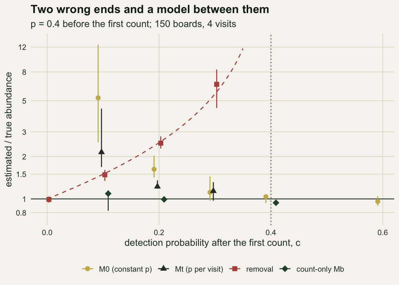
Each end has its own runaway
A ratio at an end of the scale is not a number worth quoting, because at c = 0 the M0 likelihood keeps rising as abundance grows and detection shrinks, the unbounded case described by Dennis, Morgan and Ridout (2015) and shown in the reliability post. What can be quoted is how often it happens. The rule is the ceiling check of Checking an N-mixture model made into a rate: a data set counts as a runaway when its M0 estimate at K = 160 exceeds its own estimate at K = 80 by more than 10 per cent. For the removal model the rate is the share of data sets whose totals fail the decline condition, so that no finite estimate exists at all. Both shares are over the 20 data sets of each cell.
run_tab <- do.call(rbind, lapply(c_grid, function(cc) {
  cell_rows <- tab1[tab1$c_true == cc, ]
  data.frame(c_true = cc, model = c("M0: follows the ceiling", "removal: no finite estimate"),
             share = c(mean(cell_rows$m0_hi > 1.1 * cell_rows$m0), mean(cell_rows$rem_fin == 0)))
}))
run_tab$mcse <- sqrt(run_tab$share * (1 - run_tab$share) / n_rep1)
run_at <- function(cc, k) run_tab$share[run_tab$c_true == cc][k]
k_dep <- median(tab1$m0_hi[tab1$c_true == 0] / tab1$m0[tab1$c_true == 0])
mcse_half <- sqrt(0.25 / n_rep1)
At c = 0 every M0 estimate follows the ceiling (share 1.00): doubling K from 80 to 160 multiplies the median estimate by 2.19. At c = 0.1 the share is 0.20, and from c = 0.2 upwards it is 0.00. The removal model mirrors it. Its non-finite share is 0.00 up to c = 0.3, 0.55 at c = p and 1.00 at c = 0.6. At c = p the expected totals are flat, which puts the population exactly on the boundary of the decline condition, so roughly half the data sets should fall on the wrong side; the measured share is within two Monte Carlo standard errors (at most 0.11 for 20 data sets) of one half. Between the two runaways lies a band where both models return a finite, confident and wrong estimate, and that band, not the runaway, is the dangerous part of the scale.
ggplot(run_tab, aes(c_true, share, colour = model)) +
  geom_vline(xintercept = p_det, colour = te_body, linetype = "dotted", linewidth = 0.5) +
  geom_errorbar(aes(ymin = pmax(0, share - 2 * mcse), ymax = pmin(1, share + 2 * mcse)),
                width = 0.012, linewidth = 0.5) +
  geom_line(linewidth = 0.9) + geom_point(size = 2.4) +
  scale_colour_manual(values = c(te_gold, te_rust), name = NULL) +
  scale_y_continuous(limits = c(0, 1)) +
  labs(x = "detection probability after the first count, c", y = "share of data sets",
       title = "Each simple model fails outright at one end",
       subtitle = "dotted line: c = p, where the ordinary N-mixture is the true model") +
  theme_datasheet() + theme(legend.position = "bottom")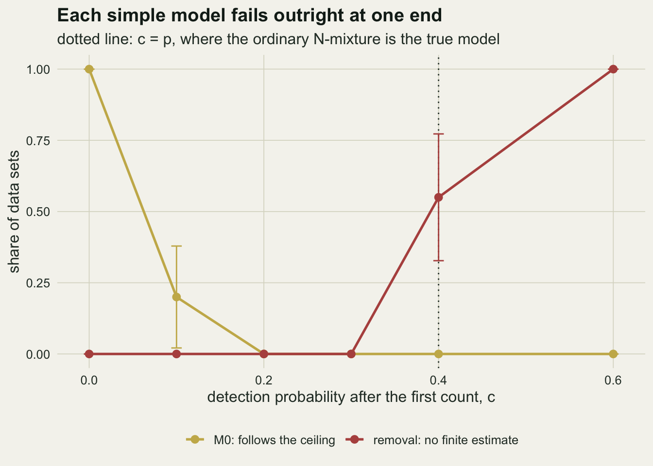
Where the counts stop telling the models apart
The large design is generous. A working survey is more like 100 boards, 3 visits and 2 animals per board, and this is where the repair has to earn its keep. The count-only Mb, M0 and Mt are fitted to 25 data sets at each of c = 0.2, 0.3 and 0.4; the last is the control, where there is no response and the extra parameter should cost something. Two questions are asked: whether the Mb median recovers abundance, and whether the data can say that Mb is needed, judged by the share of data sets in which Mb has the lowest AIC of the three.
site_w <- 100; vis_w <- 3; lam_w <- 2; c_w <- c(0.2, 0.3, 0.4); n_rep_w <- 25
set.seed(3314)
tab4 <- do.call(rbind, lapply(c_w, function(cc) do.call(rbind, lapply(seq_len(n_rep_w), function(d) {
  h <- collapse(sim_counts(site_w, lam_w, vis_w, p_det, cc))
  fb <- fit_mb(h, k_mb); f0 <- fit_m0(h, k_lo); ft <- fit_mt(h, k_lo)
  data.frame(c_true = cc, mb = fb[["lam"]] / lam_w, p_hat = fb[["p"]], c_hat = fb[["c"]],
             m0 = f0[["lam"]] / lam_w, mt = ft[["lam"]] / lam_w,
             aic_0 = 2 * f0[["nll"]] + 4, aic_t = 2 * ft[["nll"]] + 2 * (vis_w + 1),
             aic_b = 2 * fb[["nll"]] + 6)
}))))
tab4$mb_best <- tab4$aic_b < pmin(tab4$aic_0, tab4$aic_t)
s4 <- function(col, cc) cell(tab4[[col]][tab4$c_true == cc])
pick <- tapply(tab4$mb_best, tab4$c_true, mean)
pick_se <- sqrt(pick * (1 - pick) / n_rep_w)
wide_ratio <- (s4("mb", 0.4)["hi"] - s4("mb", 0.4)["lo"]) / (s4("m0", 0.4)["hi"] - s4("m0", 0.4)["lo"])
cor_lc <- sapply(c_w, function(cc) with(tab4[tab4$c_true == cc, ], cor(mb, c_hat)))
cor_lp <- sapply(c_w, function(cc) with(tab4[tab4$c_true == cc, ], cor(mb, p_hat)))
The repair holds its median. At c = 0.2 the count-only Mb gives 1.06 (10th to 90th percentile 0.88 to 1.32) where M0 gives 1.64 and Mt 1.50; c-hat has a median of 0.19. At c = 0.3 the Mb median is 0.99 against 1.14 for M0, and c-hat 0.30. What the small design costs is spread. The first visit’s mean fixes the product of abundance and p, the covariance between visits then fixes c, and abundance is read from how fast the counts of fresh animals fall, which runs through p-hat. Within a cell lambda-hat falls as p-hat rises (correlation -0.88 at c = 0.2 and -0.77 at c = 0.3) and less strongly as c-hat rises (-0.36 and -0.55): this is the ordinary N-p ridge of the N-mixture, with c riding along it. In the control cell, where M0 is the true model, the Mb 10th to 90th percentile range is 1.2 times as wide as M0’s, and its median is 1.00.
Detecting the response is the weaker link. AIC picks the count-only Mb as the best of the three models in 72 per cent of the data sets at c = 0.2, 32 per cent at c = 0.3 and 8 per cent in the control, each with a Monte Carlo standard error of up to 9 percentage points. A response that halves detection is found in most surveys of this size; the milder one at c = 0.3 is missed in 68 per cent of them, and then the analyst reports M0 or Mt and their bias. This is where identification stops in practice: not in the median of the estimator, which stays near the truth, but in the counts’ ability to say that the estimator is needed. With two visits, as shown earlier, the answer is never.
tab4$c_lab <- factor(sprintf("true c = %.1f", tab4$c_true))
tab4$c_short <- factor(sprintf("%.1f", tab4$c_true))
col_c <- c(te_rust, te_gold, te_forest)
p_ridge <- ggplot(tab4, aes(p_hat, mb, colour = c_lab)) +
  geom_hline(yintercept = 1, colour = te_body, linewidth = 0.5) +
  geom_vline(xintercept = p_det, colour = te_body, linetype = "dotted", linewidth = 0.5) +
  geom_point(size = 2, alpha = 0.85) +
  scale_colour_manual(values = col_c, name = NULL) +
  scale_y_log10(breaks = c(0.6, 0.8, 1, 1.25, 1.6, 2),
                labels = c("0.6", "0.8", "1", "1.25", "1.6", "2")) +
  labs(x = "estimated p", y = "estimated / true abundance",
       title = "The repair on a small survey", subtitle = "one point per data set") +
  theme_datasheet() + theme(legend.position = "bottom")
pick_df <- data.frame(c_short = levels(tab4$c_short), share = as.vector(pick), se = as.vector(pick_se))
p_pick <- ggplot(pick_df, aes(c_short, share, fill = c_short)) +
  geom_col(width = 0.6) +
  geom_errorbar(aes(ymin = pmax(0, share - 2 * se), ymax = pmin(1, share + 2 * se)),
                width = 0.15, linewidth = 0.5, colour = te_ink) +
  scale_fill_manual(values = col_c, guide = "none") +
  scale_y_continuous(limits = c(0, 1)) +
  labs(x = "true c", y = "share with Mb best by AIC",
       title = "Can the counts see it?", subtitle = "0.4: no response") +
  theme_datasheet()
p_ridge + p_pick + plot_layout(widths = c(1.4, 1)) + plot_annotation(theme = theme_datasheet())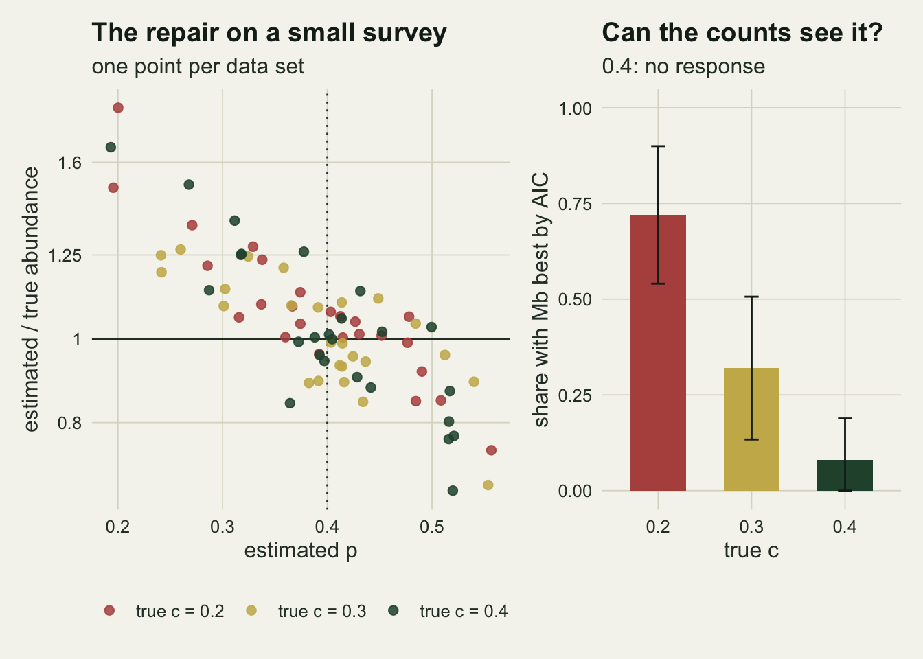
What to report
Say whether counting could have changed the animals. Turning cover objects, flushing, netting and handling all can; a count from a distance usually cannot. If it could, report the visit means, because a steady decline is the first sign, and say what the spacing of visits was: the Marsh and Goicochea result is that spacing matters for cover boards.
If an N-mixture was fitted to such counts, report the ceiling check and the removal decline condition alongside the estimate. They are cheap and they locate a survey on the scale: an M0 estimate that follows K and totals that decline steeply point towards the removal end; totals that barely decline and a stable M0 point towards the other.
Report the count-only Mb, or any behavioural-response model, together with M0 and Mt and the AIC differences, not in place of them. Its median recovered abundance across every cell measured here, but in a small survey its individual estimates spread widely, and lambda-hat trades off against p-hat as in any N-mixture. Give p-hat and c-hat with their intervals, because the abundance estimate is conditional on both.
With two visits, do not report a behavioural-response analysis as a finding. The two-visit counts fit a time effect and a counting response equally well, so the abundance estimate is set by the assumption chosen, and the report should say which assumption that was.
Honest limits
The response here attaches only to counted animals and lasts for the rest of the survey. Real disturbance is messier. Turning a board may also displace animals that were under it but missed, which is a visit-level effect of the kind the reliability post simulates, and a displaced animal may drift back between visits days apart, so that c recovers towards p. Marsh and Goicochea did not follow individuals, so their count reduction cannot be split into the part that fell on animals already handled; the size of c in any real survey is not known from this post.
Everything is at p = 0.4, with two designs and the replication the knitting budget allowed: 20 data sets per cell for M0 and the removal model, 8 for Mt, 4 for the count-only Mb in the large design and 25 in the working design. The Mb results in the large design are ranges over four fits, not percentiles. Other values of p and other numbers of visits were not measured, and the crossing point between M0 and the removal model, which lies between c = 0.1 and c = 0.2 here, will move with them.
The count-only Mb assumes a Poisson abundance layer and closure. With a negative binomial layer the ordinary N-mixture already has a weakly identified dispersion parameter, and adding c on top of it is likely to widen the ridge seen in the working design. The ceiling of 20 for the Mb fits is ample at the abundances used here and would have to rise for denser sites, at a cost in time that grows with the square of the ceiling.
A design repair was not measured. Holding every counted animal until the last visit forces c to zero and makes the removal model exact; whether that is cheaper than more visits and a behavioural-response model depends on the animal and the permit, and this post has no numbers on it.
References
Royle JA 2004 Biometrics 60(1):108-115 (10.1111/j.0006-341X.2004.00142.x)
Dorazio RM, Jelks HL, Jordan F 2005 Biometrics 61(4):1093-1101 (10.1111/j.1541-0420.2005.00360.x)
Marsh DM, Goicochea MA 2003 Journal of Herpetology 37(3):460-466 (10.1670/98-02A)
Dennis EB, Morgan BJT, Ridout MS 2015 Biometrics 71(1):237-246 (10.1111/biom.12246)
Link WA, Schofield MR, Barker RJ, Sauer JR 2018 Ecology 99(7):1547-1551 (10.1002/ecy.2362)