library(ggplot2)
library(patchwork)

te_paper  <- "#f5f4ee"
te_ink    <- "#16241d"
te_body   <- "#2c3a31"
te_forest <- "#275139"
te_rust   <- "#b5534e"
te_gold   <- "#c9b458"
te_line   <- "#dad9ca"

theme_datasheet <- function() {
  theme_minimal(base_size = 12) +
    theme(plot.background  = element_rect(fill = te_paper, colour = NA),
          panel.background = element_rect(fill = te_paper, colour = NA),
          panel.grid.major = element_line(colour = te_line, linewidth = 0.3),
          panel.grid.minor = element_blank(),
          text             = element_text(colour = te_body),
          plot.title       = element_text(colour = te_ink, face = "bold"),
          plot.subtitle    = element_text(colour = te_body),
          axis.text        = element_text(colour = te_body))
}Open N-mixture models and the detection trap
R
abundance
imperfect detection
population dynamics
simulation
ecology tutorial
Open N-mixture models in R: a hand-coded forward algorithm fits survival and recruitment to repeat counts, and tests which detection errors the visits catch.
Sixty farm ponds, each visited on three nights every spring for five years, and at each visit a surveyor walks the margin with a torch and counts adult newts. Nobody marks anything. At the end of the fifth season the table holds nine hundred counts, and the questions asked of it are about change: whether the ponds are gaining animals, how many adults survive from one spring to the next, and how many new ones arrive.
The binomial N-mixture model turns the three counts of one season into an abundance, by treating the spread among repeat visits as information about detection (Royle 2004). Dail and Madsen extended that idea to a population that is open between seasons. The abundance in the first year is Poisson, as in the closed model. Between years each animal survives with probability omega, a Poisson number of recruits with mean gamma is added, and within each year the three visits are binomial counts of whatever is there. The seasons are chained, and the counts alone are asked to give survival and recruitment.
The chaining is where the detection model starts to matter in a new way. N-mixture reliability and the detection trade-off measured what hidden detection heterogeneity does to abundance in a closed population; across seasons the same kind of error lands in survival and recruitment, which are usually the reason the open model was fitted in the first place. The likelihood is a forward algorithm of exactly the kind built in Dynamic occupancy: colonisation and extinction, with the two occupancy states replaced by every abundance from zero to a ceiling.
Two detection problems are simulated here, and they behave in opposite ways. The first is a year-to-year drift in detection, the counting version of the effort drift in Reporting rates and effort drift and of the observer steps in Observer effects and the first-year dip. Neither of those posts uses repeat visits within a season as information about detection, so a change in detection can be handled there only through a recorded covariate: list length in the first, which removes part of the false trend from some kinds of drift and none of it from others, and a first-year term for each new observer in the second, which removes the bias that post measures. Here the three visits per season are the extra information, and the question is whether a detection model that is allowed to change by year uses it. The second problem is detection that falls as abundance rises, which year effects can absorb only in part.
The model and its forward likelihood
The simulation follows the constant dynamics of Dail and Madsen. Initial abundance at each pond is Poisson with mean lambda. From one year to the next the survivors are a binomial draw from last year’s animals with probability omega, and the recruits are Poisson with mean gamma, whatever the pond already holds. Each of the three visits counts every animal present independently with probability p. The design constants are fixed before anything is fitted: 60 ponds, five years, three visits, lambda 5, omega 0.7 and gamma 2.
Three of those numbers set the trend the post is about. The expected abundance obeys m(t) = omega m(t - 1) + gamma, starting from lambda, so the expected abundance in year five divided by that in year one is a function of the three rates alone. That ratio, computed from fitted rates, is what “trend” means below. The realised ratio of mean abundance in the simulated ponds is printed beside it as a check on the simulation, not as the target.
n_site  <- 60
n_year  <- 5
n_visit <- 3
lambda_true <- 5
omega_true  <- 0.7
gamma_true  <- 2
k_max <- 35

trend_of <- function(lambda, omega, gamma, n_yr = n_year) {
  m_t <- lambda
  for (tt in 2:n_yr) m_t <- c(m_t, omega * m_t[tt - 1] + gamma)
  m_t[n_yr] / m_t[1]
}
trend_true <- trend_of(lambda_true, omega_true, gamma_true)

sim_abund <- function(n_s = n_site, n_yr = n_year, lambda = lambda_true,
                      omega = omega_true, gamma = gamma_true) {
  abund <- matrix(0L, n_s, n_yr)
  abund[, 1] <- rpois(n_s, lambda)
  for (tt in 2:n_yr)
    abund[, tt] <- rbinom(n_s, abund[, tt - 1], omega) + rpois(n_s, gamma)
  abund
}

sim_counts <- function(abund, p_fun, n_v = n_visit) {
  counts <- array(0L, c(dim(abund), n_v))
  for (tt in seq_len(ncol(abund))) {
    p_now <- p_fun(tt, abund[, tt])
    for (j in seq_len(n_v))
      counts[, tt, j] <- rbinom(nrow(abund), abund[, tt], p_now)
  }
  counts
}

# everything in the binomial likelihood that does not involve p,
# computed once per data set: log choose terms, and -Inf where N < max count
prep_counts <- function(counts, K) {
  n_s <- dim(counts)[1]; n_yr <- dim(counts)[2]
  n_vals <- 0:K
  n_mat  <- matrix(n_vals, n_s, K + 1, byrow = TRUE)
  log_ch <- array(0, c(n_s, n_yr, K + 1))
  for (tt in seq_len(n_yr)) {
    for (j in seq_len(dim(counts)[3]))
      log_ch[, tt, ] <- log_ch[, tt, ] + lchoose(n_mat, counts[, tt, j])
    too_small <- outer(apply(counts[, tt, , drop = FALSE], 1, max), n_vals, ">")
    log_ch[, tt, ][too_small] <- -Inf
  }
  list(K = K, n_vals = n_vals, n_s = n_s, n_yr = n_yr, n_v = dim(counts)[3],
       y_sum = apply(counts, c(1, 2), sum), log_ch = log_ch)
}

# p models: "const", "year" (logit-linear in year), "abund" (logit-linear in N)
det_prob <- function(par, tt, dat, pmode) {
  mid <- (dat$n_yr + 1) / 2
  eta <- switch(pmode,
    const = rep(par[4], dat$K + 1),
    year  = rep(par[4] + par[5] * (tt - mid), dat$K + 1),
    abund = par[4] + par[5] * (dat$n_vals - 6))
  matrix(plogis(eta), dat$n_s, dat$K + 1, byrow = TRUE)
}

nll_dm <- function(par, dat, pmode) {
  lambda <- exp(par[1]); omega <- plogis(par[2]); gamma <- exp(par[3])
  n_vals <- dat$n_vals
  surv  <- outer(n_vals, n_vals, function(n, s) dbinom(s, n, omega))
  recr  <- outer(n_vals, n_vals, function(s, m) ifelse(m >= s, dpois(pmax(m - s, 0), gamma), 0))
  trans <- surv %*% recr
  n_obs <- matrix(dat$n_v * n_vals, dat$n_s, dat$K + 1, byrow = TRUE)
  emit <- function(tt) {
    p_mat <- det_prob(par, tt, dat, pmode)
    exp(dat$log_ch[, tt, ] + dat$y_sum[, tt] * log(p_mat) +
          (n_obs - dat$y_sum[, tt]) * log1p(-p_mat))
  }
  alpha  <- matrix(dpois(n_vals, lambda), dat$n_s, dat$K + 1, byrow = TRUE) * emit(1)
  loglik <- 0
  for (tt in 2:dat$n_yr) {
    scale_t <- rowSums(alpha)
    loglik  <- loglik + sum(log(scale_t))
    alpha   <- ((alpha / scale_t) %*% trans) * emit(tt)
  }
  value <- -(loglik + sum(log(rowSums(alpha))))
  if (is.finite(value)) value else 1e10
}

fit_dm <- function(dat, pmode) {
  start_par <- c(log(5), qlogis(0.6), log(1.5), 0, if (pmode != "const") 0)
  opt <- optim(start_par, nll_dm, dat = dat, pmode = pmode, method = "BFGS")
  est <- c(lambda = exp(opt$par[1]), omega = plogis(opt$par[2]),
           gamma = exp(opt$par[3]), p_int = plogis(opt$par[4]),
           p_slope = if (pmode == "const") NA else opt$par[5])
  c(est, trend = trend_of(est[["lambda"]], est[["omega"]], est[["gamma"]]),
    aic = 2 * opt$value + 2 * length(start_par), conv = opt$convergence)
}
The survival matrix and the recruitment matrix are multiplied once per likelihood call to give the transition matrix from last year’s abundance to this year’s. Each pond carries a vector of probabilities over abundances from zero to K, and all sixty vectors are rows of one matrix, so the forward step is a single matrix product per year rather than a loop over ponds. Each row is rescaled to sum to one before the product, and the log of the scale factors adds up to the log likelihood.
A forward algorithm that is wrong in a subtle place still returns a number, so the first check is against the sum it replaces. With two ponds, two years, two visits and a ceiling of twelve, the likelihood can be written as a double sum over the abundance in both years, with the survivor count summed inside, and computed with no recursion at all.
set.seed(2011)
tiny_abund  <- sim_abund(n_s = 2, n_yr = 2)
tiny_counts <- sim_counts(tiny_abund, function(tt, n) rep(0.6, length(n)), n_v = 2)
k_tiny   <- 12
par_test <- c(log(4), qlogis(0.65), log(1.8), qlogis(0.55))

brute_ll <- 0
for (i in 1:2) {
  site_sum <- 0
  for (n1 in 0:k_tiny) for (n2 in 0:k_tiny) {
    s_vals <- 0:min(n1, n2)
    p_tr <- sum(dbinom(s_vals, n1, plogis(par_test[2])) *
                  dpois(n2 - s_vals, exp(par_test[3])))
    site_sum <- site_sum + dpois(n1, exp(par_test[1])) * p_tr *
      prod(dbinom(tiny_counts[i, 1, ], n1, plogis(par_test[4]))) *
      prod(dbinom(tiny_counts[i, 2, ], n2, plogis(par_test[4])))
  }
  brute_ll <- brute_ll + log(site_sum)
}
forward_ll <- -nll_dm(par_test, prep_counts(tiny_counts, k_tiny), "const")
ll_gap <- abs(brute_ll - forward_ll)
The brute-force log likelihood is -13.0376274662 and the forward algorithm gives -13.0376274662; the absolute difference is 3.55e-15.
The second check is the ceiling. Abundance has no upper limit, and K = 35 truncates the sum. Every replicate below stops if any simulated abundance comes within five of the ceiling. On one control data set the fit is repeated with K = 60.
set.seed(2012)
k_abund  <- sim_abund()
k_counts <- sim_counts(k_abund, function(tt, n) rep(0.5, length(n)))
time_35 <- system.time(fit_35 <- fit_dm(prep_counts(k_counts, k_max), "const"))[["elapsed"]]
time_60 <- system.time(fit_60 <- fit_dm(prep_counts(k_counts, 60), "const"))[["elapsed"]]
k_diff  <- max(abs(fit_35[c("lambda", "omega", "gamma", "p_int")] -
                   fit_60[c("lambda", "omega", "gamma", "p_int")]))
k_maxN  <- max(k_abund)
k_ll    <- -nll_dm(c(log(5), qlogis(0.7), log(2), 0), prep_counts(k_counts, 60), "const") +
  nll_dm(c(log(5), qlogis(0.7), log(2), 0), prep_counts(k_counts, k_max), "const")
The largest simulated abundance in that data set is 13. Between K = 35 and K = 60 the largest change in any of lambda, omega, gamma and p prints as 0.000000, and the change in log likelihood at the true rates prints as 0.000000: the probability above the lower ceiling is too small to register. The fit took 0.08 seconds at K = 35 and 0.15 seconds at K = 60 on the machine that built this page.
Counts alone recover survival and recruitment
The replicate study uses common random numbers. For each of 60 replicates one abundance history is drawn, and the three detection scenarios below all count that same set of animals. The differences between scenarios are then differences in detection, not in which ponds happened to grow.
n_rep <- 60
set.seed(3101)
abund_list <- lapply(seq_len(n_rep), function(r) sim_abund())
max_abund  <- max(sapply(abund_list, max))
stopifnot(max_abund < k_max - 5)
realised <- sapply(abund_list, function(a) mean(a[, n_year]) / mean(a[, 1]))

run_scenario <- function(p_fun, models, seed) {
  set.seed(seed)
  rows <- lapply(seq_len(n_rep), function(r) {
    cnt <- sim_counts(abund_list[[r]], p_fun)
    dat <- prep_counts(cnt, k_max)
    cnt_mean <- setNames(apply(cnt, 2, mean), paste0("count", seq_len(n_year)))
    do.call(rbind, lapply(models, function(m)
      data.frame(rep = r, model = m, t(fit_dm(dat, m)), t(cnt_mean))))
  })
  do.call(rbind, rows)
}

med_mcse <- function(x, n_boot = 1000) {
  sd(replicate(n_boot, median(sample(x, replace = TRUE))))
}

study_time <- system.time(
  ctl <- run_scenario(function(tt, n) rep(0.5, length(n)), c("const", "year"), 3102)
)[["elapsed"]]
ctl_c <- ctl[ctl$model == "const", ]
set.seed(3103)
ctl_mcse <- sapply(c("omega", "gamma", "trend"), function(v) med_mcse(ctl_c[[v]]))
With detection at a constant 0.5 and the constant-p model fitted, the median estimates over 60 data sets are lambda 4.97, omega 0.705 (bootstrap Monte Carlo standard error 0.009) and gamma 1.99 (0.04), against 5, 0.7 and 2. The fitted trend has a median of 1.247 (0.020) against 1.253 implied by the design, and the realised ratio of mean abundance in the simulated ponds has a median of 1.246. The spread is wide: the middle half of omega estimates runs from 0.65 to 0.74, which is what five years of unmarked counts at sixty ponds can say about survival. The largest abundance in any replicate was 19, well inside the ceiling.
A drift in detection, and the replicates that catch it
Now the torch gets worse. Detection falls on the logit scale by 0.35 per year, from 0.75 in the first spring to 0.43 in the fifth, perhaps because the water clouds or the surveyor changes. The newts are exactly the ones counted in the control scenario.
p_drift <- function(tt, n) rep(plogis(0.4 - 0.35 * (tt - 3)), length(n))
dft <- run_scenario(p_drift, c("const", "year"), 3104)
dft_c <- dft[dft$model == "const", ]
dft_y <- dft[dft$model == "year", ]
daic_drift <- dft_c$aic - dft_y$aic
daic_ctl   <- ctl_c$aic - ctl[ctl$model == "year", "aic"]
set.seed(3105)
dft_mcse <- sapply(list(c_tr = dft_c$trend, y_tr = dft_y$trend,
                        c_om = dft_c$omega, y_om = dft_y$omega), med_mcse)
raw_ratio <- median(dft_c$count5 / dft_c$count1)
n_decline <- sum(dft_c$trend < 1)
count_cols <- paste0("count", seq_len(n_year))
true_mean <- rowMeans(sapply(abund_list, colMeans))
count_tab <- rbind(
data.frame(scenario = "constant detection", year = 1:n_year,
what = "mean count per visit", value = colMeans(ctl_c[, count_cols])),
data.frame(scenario = "detection drifts down", year = 1:n_year,
what = "mean count per visit", value = colMeans(dft_c[, count_cols])),
data.frame(scenario = "constant detection", year = 1:n_year,
what = "mean true abundance", value = true_mean),
data.frame(scenario = "detection drifts down", year = 1:n_year,
what = "mean true abundance", value = true_mean))
count_tab$scenario <- factor(count_tab$scenario, levels = unique(count_tab$scenario))
ggplot(count_tab, aes(year, value, colour = what)) +
geom_line(linewidth = 0.9) + geom_point(size = 2) +
facet_wrap(~ scenario) +
scale_colour_manual(values = c(te_rust, te_forest), name = NULL) +
scale_y_continuous(limits = c(0, NA)) +
labs(x = "year", y = "animals per pond",
title = "The counts and the animals",
subtitle = "averages over all replicate data sets") +
theme_datasheet() + theme(legend.position = "bottom")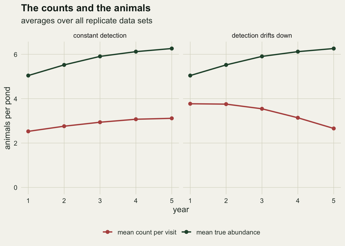
Fitted with constant detection, the model has to explain counts that fall while the animals rise. It does so with the rates. The median omega drops to 0.651 (0.009), median gamma to 1.67, median lambda rises to 6.24, and the median fitted trend is 0.807 (0.012) where the truth is 1.253. The fitted trend is below one in 60 of the 60 data sets: a growing population reported as shrinking. The raw counts themselves fall to a median ratio of 0.705 between the last and first year, so the constant-p model is not inventing the decline; it is believing the counts.
The same data carry the evidence against that belief. Within each spring the three visits pin down detection for that spring, and a model in which logit p changes linearly by year can use it. That model returns a median omega of 0.706 (0.008), gamma 1.97, lambda 4.99, and a trend of 1.241 (0.012). AIC chooses it without hesitation: the AIC of the constant model minus that of the year model has a median of 35.7 and a minimum of 7.6. In the control scenario, where the extra slope is not needed, the same difference has a median of -1.6 and is below two in 92 per cent of data sets.
The reporting-rate and observer posts handle a change in detection through a recorded covariate. Here no covariate was recorded, and the drift is estimated from the counts themselves only because each season was counted more than once. Take away the replicate visits, and any covariate that tracks the change, and a year effect in detection is indistinguishable from a year effect in abundance.
Detection that depends on abundance
The third scenario returns detection to no trend in time but makes it depend on how many newts are in the pond: logit p = 0.6 - 0.12 (N - 6), so a pond with two adults is counted with probability 0.75 per animal and one with fifteen with probability 0.38. Crowded margins, animals hidden behind one another, and a surveyor who stops counting carefully at a busy pond all push in that direction. Three models are fitted: constant p, p changing by year, and p changing with abundance, which is the true form. The last needs no new machinery, because the forward algorithm already carries a probability for every abundance and the emission can use a different p in each column.
p_dens <- function(tt, n) plogis(0.6 - 0.12 * (n - 6))
den <- run_scenario(p_dens, c("const", "year", "abund"), 3107)
den_c <- den[den$model == "const", ]
den_y <- den[den$model == "year", ]
den_a <- den[den$model == "abund", ]
daic_cy <- den_c$aic - den_y$aic
daic_ca <- den_c$aic - den_a$aic
set.seed(3108)
den_mcse <- sapply(list(c_om = den_c$omega, c_ga = den_c$gamma, c_tr = den_c$trend,
                        a_om = den_a$omega, a_ga = den_a$gamma), med_mcse)
eq_mean <- function(fit) median(fit$gamma / (1 - fit$omega))
all_fits <- rbind(ctl, dft, den)
n_fits   <- nrow(all_fits)
n_noconv <- sum(all_fits$conv != 0)
p_avg <- sapply(seq_len(n_year), function(tt)
  mean(sapply(abund_list, function(a) sum(a[, tt] * p_dens(tt, a[, tt])) / sum(a[, tt]))))
daic_wilcox <- wilcox.test(daic_cy, daic_ctl)$p.value
Under constant p the rates move again, but in the other direction: median omega 0.799 (0.006) and median gamma 1.35 (0.04). Initial abundance is barely touched (median lambda 5.09), and the median trend is 1.190 (0.012) against 1.253. The year model does no better on the rates, omega 0.805 and gamma 1.37, but it does recover the trend, with a median of 1.255. Detection has no time term in this scenario, yet the ponds fill up over the five years, so detection averaged over the animals present falls a little each spring, from 0.643 in the first to 0.608 in the fifth, and a slope on year absorbs that part of the error. AIC mostly cannot choose between the two models: the constant model minus the year model has a median of -0.9, the year model is ahead by more than two units in 18 per cent of data sets (Monte Carlo standard error 5 points) and the constant model in 0 per cent. In the control scenario, where the year slope is truly zero, the year model is ahead by more than two in 8 per cent, and a Wilcoxon rank-sum test on the two sets of AIC differences gives p = 0.014: a small, detectable lean towards the year model, not a verdict in any one data set.
rate_tab <- rbind(cbind(ctl, scenario = "constant\ndetection"),
                  cbind(dft, scenario = "detection\ndrifts down"),
                  cbind(den, scenario = "detection falls\nwith abundance"))
rate_tab$scenario <- factor(rate_tab$scenario, levels = unique(rate_tab$scenario))
rate_tab$model <- factor(rate_tab$model, levels = c("const", "year", "abund"),
                         labels = c("p constant", "p by year", "p by abundance"))
rate_plot <- function(v, truth, lab) {
  ggplot(rate_tab, aes(scenario, .data[[v]], colour = model)) +
    geom_hline(yintercept = truth, linetype = "dashed", colour = te_body, linewidth = 0.5) +
    geom_boxplot(outlier.shape = NA, fill = te_paper, width = 0.7,
                 position = position_dodge(0.8), linewidth = 0.5) +
    geom_point(position = position_jitterdodge(jitter.width = 0.15, dodge.width = 0.8,
                                               seed = 1), size = 0.7, alpha = 0.5) +
    scale_colour_manual(values = c(te_rust, te_gold, te_forest), name = NULL, drop = FALSE) +
    labs(x = NULL, y = lab) +
    theme_datasheet() + theme(legend.position = "bottom")
}
(rate_plot("omega", omega_true, "apparent survival, omega") + labs(title = "Survival") |
   rate_plot("gamma", gamma_true, "recruits per pond, gamma") + labs(title = "Recruitment")) +
  plot_layout(guides = "collect") +
  plot_annotation(theme = theme_datasheet() + theme(legend.position = "bottom"))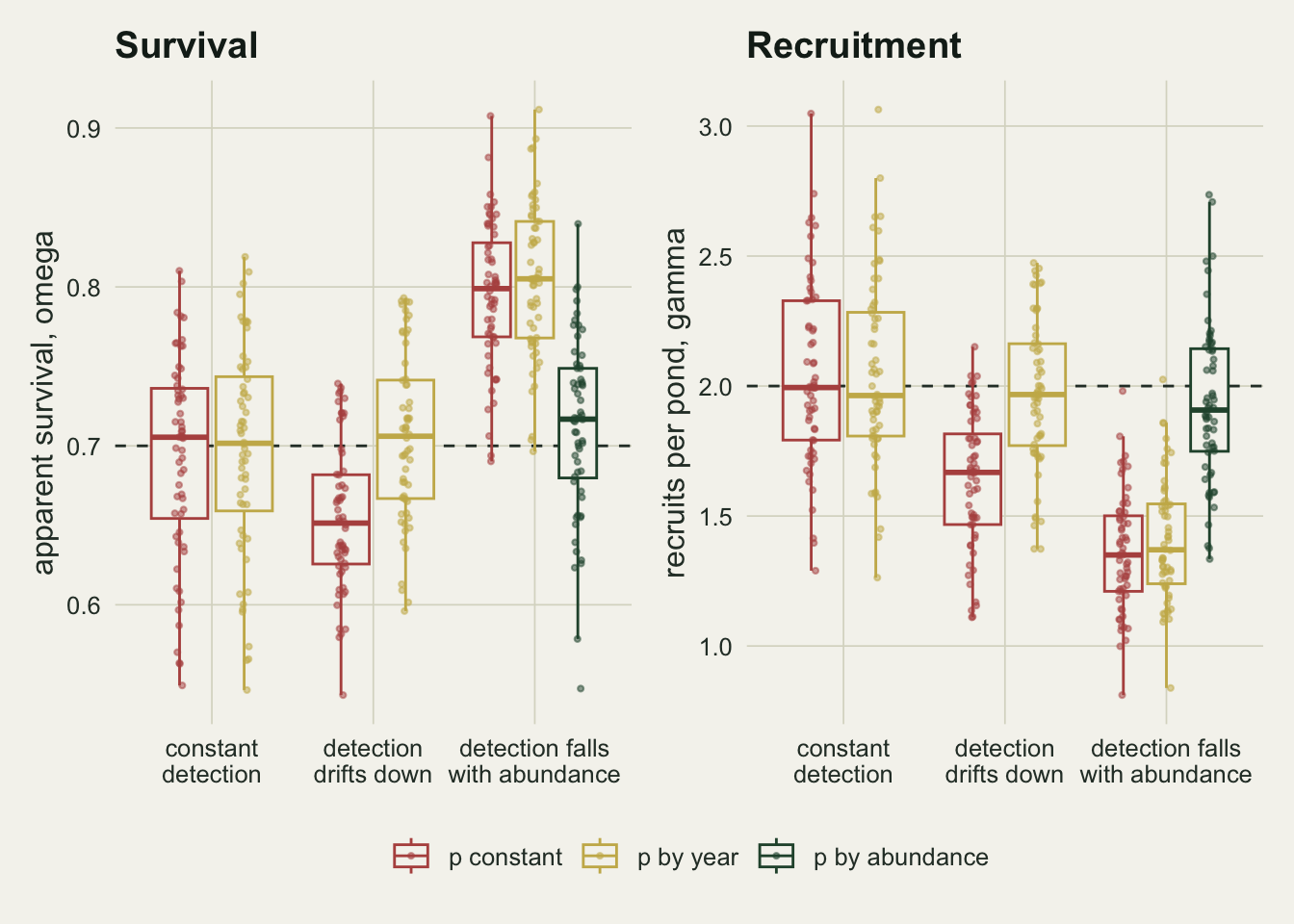
The replicate visits are not powerless against this error; they are powerless against it only when the detection model offers the wrong kind of flexibility. The model with p on abundance, given the logit-linear form the simulation used, returns median omega 0.717 (0.007), gamma 1.91 (0.04) and a slope on abundance of -0.121 against the true -0.12, with the middle half of slope estimates between -0.136 and -0.109. Its AIC is lower than the constant model’s in 60 of the 60 data sets, by a median of 23.8. The information comes from the spread of the repeat visits. For a binomial count the variance among visits is the mean count times one minus p, so a pond whose visits scatter widely around their mean is one where detection is low. When detection falls with abundance, the busier ponds scatter more than their counts alone would suggest, and a p that depends on N is fitted to exactly that pattern.
Survival and recruitment trade along one line
Why the trend survives when the rates do not is visible in the fitted values themselves. The counts constrain the level the ponds are heading towards better than the speed at which they get there, so gamma divided by one minus omega is held close to fixed, and an error in omega is paid for by gamma along that line.
eq_true <- gamma_true / (1 - omega_true)
eq_tab <- data.frame(
  fit = c("control, p constant", "drift, p constant", "drift, p by year",
          "density, p constant", "density, p by abundance", "density, p by year"),
  eq  = c(eq_mean(ctl_c), eq_mean(dft_c), eq_mean(dft_y), eq_mean(den_c), eq_mean(den_a),
          eq_mean(den_y)))
cor_den <- cor(qlogis(den_c$omega), log(den_c$gamma))
cor_ctl <- cor(qlogis(ctl_c$omega), log(ctl_c$gamma))
eq_iqr_den <- IQR(den_c$gamma / (1 - den_c$omega))
The median implied equilibrium, gamma / (1 - omega), is 6.67 in the control fits, 6.66 under density-dependent detection with constant p and 6.68 with p on abundance, against a true 6.67. The year model breaks the pattern under the same detection error: its median equilibrium is 7.20, so under this error the ratio is not the same across detection models. The drift does not follow the line either: fitted with constant p it gives 4.68 (and 6.68 with p by year), because the counts in the last seasons really are lower, and the constant model takes the lower level as the equilibrium the ponds are heading for. Across the density replicates fitted with constant p, logit omega and log gamma correlate at -0.93, against -0.88 in the control fits with no detection error at all: the ridge is a property of five years of unmarked counts, and the error slides the estimates along it rather than creating it.
ridge_tab <- rbind(data.frame(model = "p constant", den_c[, c("omega", "gamma")]),
                   data.frame(model = "p by abundance", den_a[, c("omega", "gamma")]))
om_seq <- seq(0.45, 0.95, by = 0.005)
ggplot(ridge_tab, aes(omega, gamma, colour = model)) +
  geom_line(data = data.frame(omega = om_seq, gamma = eq_true * (1 - om_seq)),
            aes(omega, gamma), inherit.aes = FALSE,
            colour = te_body, linetype = "dashed", linewidth = 0.6) +
  geom_point(size = 2, alpha = 0.8) +
  annotate("point", x = omega_true, y = gamma_true, shape = 4, size = 5,
           stroke = 1.4, colour = te_ink) +
  scale_colour_manual(values = c(te_forest, te_rust), name = NULL) +
  coord_cartesian(xlim = range(c(ridge_tab$omega, 0.6)), ylim = range(c(ridge_tab$gamma, 1))) +
  labs(x = "apparent survival, omega", y = "recruits per pond, gamma",
       title = "Survival and recruitment trade along one line",
       subtitle = "detection falls with abundance; dashed: gamma / (1 - omega) at its true value") +
  theme_datasheet() + theme(legend.position = "bottom")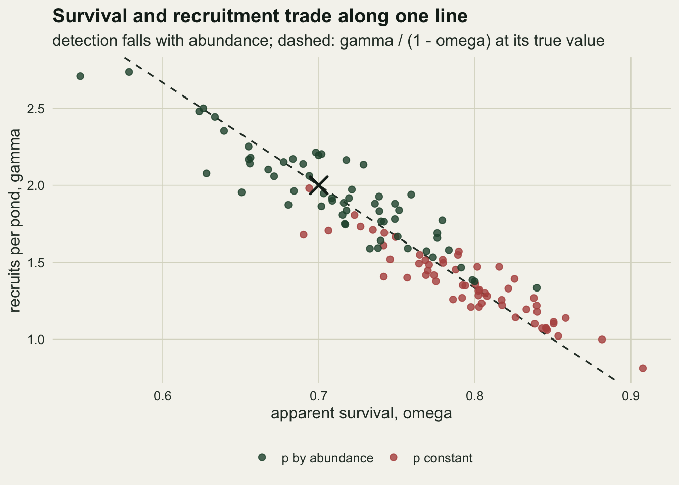
ggplot(rate_tab, aes(scenario, trend, colour = model)) +
  geom_hline(yintercept = trend_true, linetype = "dashed", colour = te_body, linewidth = 0.5) +
  geom_hline(yintercept = 1, colour = te_line, linewidth = 0.8) +
  geom_boxplot(outlier.shape = NA, fill = te_paper, width = 0.7,
               position = position_dodge(0.8), linewidth = 0.5) +
  geom_point(position = position_jitterdodge(jitter.width = 0.15, dodge.width = 0.8, seed = 1),
             size = 0.7, alpha = 0.5) +
  scale_colour_manual(values = c(te_rust, te_gold, te_forest), name = NULL) +
  labs(x = NULL, y = "fitted E[N5] / E[N1]",
       title = "The trend under three detection errors",
       subtitle = "dashed: the trend implied by the true rates; solid grey: no change") +
  theme_datasheet() + theme(legend.position = "bottom")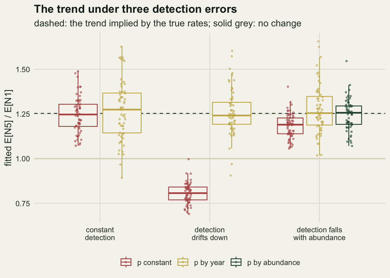
iqr_of <- function(x) diff(quantile(x, c(0.25, 0.75)))
iqr_ctl_c <- iqr_of(ctl_c$trend)
iqr_ctl_y <- iqr_of(ctl[ctl$model == "year", "trend"])
iqr_den_a <- iqr_of(den_a$trend)
The figure puts the three scenarios side by side. Only the drift fitted with constant p moves the typical trend across one (2 control fits and 2 drift fits under the year model also fall below it, out of 60 each); under density-dependent detection the constant-p trend sits a little low while the rates in the survival and recruitment figure are far off. Flexibility in detection is not free: in the control scenario the interquartile range of the fitted trend is 0.124 under constant p and 0.223 under the year model, which spends part of the information in the counts on a slope that is zero. The abundance model in the density scenario has an interquartile range of 0.103.
Across all 420 fits in the three scenarios, 0 ended with a non-zero convergence code from optim. The control study alone took 10 seconds for 120 fits on the machine that built this page.
What to report
Report the trend as a named quantity. Here it was the expected abundance in the last year over the first, computed from the fitted lambda, omega and gamma; a reader cannot tell that apart from a ratio of raw counts or of realised site abundances unless the methods say which. In the drift scenario the three differ completely: the raw counts fell to a median ratio of 0.705, the constant-p fit gave 0.807 and the year fit gave 1.241.
Fit more than one detection model and print the AIC table, and let the alternatives include detection on abundance, not only detection on time and covariates. In this simulation the year model and the constant model were mostly tied under density-dependent detection (the year model ahead by more than two AIC units in 18 per cent of data sets), and the year model recovered the trend while leaving survival and recruitment as far off as the constant model did; a reader shown only that pair would have read the problem, if at all, as a drift in time. The model that found the problem, given the true logit-linear shape, was one line of code inside the emission; how it fares with a wrong shape was not measured.
Print gamma / (1 - omega) beside the two rates. Its agreement here is a median property over replicates, not a guarantee in one data set: across the density replicates fitted with constant p its interquartile range was 0.69, and the year model moved the median to 7.20. Where it agrees across detection models while omega and gamma do not, the counts have identified the level of the population and not how it turns over, and the rates should be reported as conditional on the detection model rather than as findings about survival. Under density-dependent detection with constant p the median equilibrium was within 0.01 of the truth while median omega was off by 0.099.
State the ceiling K, the largest count, and the result of refitting at a higher K, and state how many fits failed to converge. None of these costs more than a sentence, and a missing K check is the first thing a reviewer of an N-mixture paper asks about.
Honest limits
Both rescues were handed the true functional form. The drift was linear on the logit scale and the year model was linear on the logit scale; detection fell with abundance on the logit scale and the abundance model assumed exactly that, centred where the simulation centred it. A real detection pattern would be some other curve, and how much of the rescue survives a wrong curve was not measured. A separate p for each year would cover any drift at the cost of three more parameters here; nothing comparable exists for abundance, because the abundance effect has to be given a shape.
The abundance model reads detection from the spread among repeat visits, and that reading depends on the counts being binomial given N. Extra variation among visits, of the beta-binomial kind simulated in the reliability post, also widens that spread, and it would be read as low detection at busy ponds or as low detection overall. The two errors were not simulated together, and in combination the abundance slope may be far less clean than the median of -0.121 found here.
Only one set of rates was simulated, with lambda 5, omega 0.7, gamma 2, sixty ponds and five years. The populations were small and never approached the ceiling, so the K check says nothing about ponds holding hundreds of animals, where K has to be much larger and each fit correspondingly slower. With fewer years the survival and recruitment rates are less well separated and the ridge in the last figure would be longer; with a population far from equilibrium in the first year it would be shorter. Neither was tried.
The dynamics are the simplest Dail and Madsen offer: constant rates, recruitment that ignores the animals already present, no site or year covariates on survival or recruitment, and no movement between ponds. Hostetler and Chandler add density-dependent forms such as the Ricker and Gompertz models, among other extensions. Each of those adds parameters that compete with detection for the same information, so the errors measured here are more likely to grow than to shrink in a richer model.
Only point estimates were examined. Standard errors, interval coverage and the behaviour of likelihood ratio tests between detection models were not, and a biased omega with an honest-looking interval is the more dangerous output. The AIC comparisons rest on 60 replicates per scenario, which separates a median difference of 23.8 from zero easily but leaves a Monte Carlo standard error of several points on the shares quoted above. Within each season the population was closed by construction; in real ponds animals arrive and leave between the three nights, and Barker and colleagues argue that counts alone carry little information for checking assumptions of this kind.
References
Dail D, Madsen L 2011 Biometrics 67(2):577-587 (10.1111/j.1541-0420.2010.01465.x)
Royle JA 2004 Biometrics 60(1):108-115 (10.1111/j.0006-341X.2004.00142.x)
Hostetler JA, Chandler RB 2015 Ecology 96(6):1713-1723 (10.1890/14-1487.1)
Barker RJ, Schofield MR, Link WA, Sauer JR 2018 Biometrics 74(1):369-377 (10.1111/biom.12734)