library(ggplot2)

te_paper  <- "#f5f4ee"
te_ink    <- "#16241d"
te_body   <- "#2c3a31"
te_forest <- "#275139"
te_rust   <- "#b5534e"
te_gold   <- "#c9b458"
te_line   <- "#dad9ca"

theme_datasheet <- function() {
  theme_minimal(base_size = 12) +
    theme(plot.background  = element_rect(fill = te_paper, colour = NA),
          panel.background = element_rect(fill = te_paper, colour = NA),
          panel.grid.major = element_line(colour = te_line, linewidth = 0.3),
          panel.grid.minor = element_blank(),
          text             = element_text(colour = te_body),
          plot.title       = element_text(colour = te_ink, face = "bold"),
          plot.subtitle    = element_text(colour = te_body),
          axis.text        = element_text(colour = te_body))
}Observer effects and the first-year dip
R
monitoring
trend
GLM
observer effects
ecology tutorial
Adding an observer effect to a route count trend turns a novice first-year deficit into a spurious increase. Measuring the bias and the one-term fix in R.
A breeding bird route is forty stops along a country road, driven once each June by a volunteer who counts every bird heard or seen in three minutes at each stop. The same route is run for decades, but not by the same person. Volunteers move house, retire, lose their hearing for high song, and hand the route to someone new. A national scheme ends up with a table in which every route has a string of observers, each of whom covers it for a handful of years before the next one arrives.
Two things about that table are well documented. Observers differ from one another in what they count, and the trend analyses of the North American Breeding Bird Survey carry observer identity for that reason: Sauer, Peterjohn and Link (1994) found observer differences in half of the species they examined and, for many species, observers in later years counting more birds than those in earlier years, which pushes a trend fitted without observers upwards. And an observer’s first year on a route tends to be low: they are learning the stops, the local birds and the pace of the count. Kendall, Peterjohn and Sauer (1996) tested this directly and found that removing each observer’s first year from the route regression lowered the unweighted trend estimate for 415 of 459 species.
The direction of that change is the subject of this post. A lower trend after deleting the first years means that the first years had been pushing trends up. That is not the intuitive direction. The intuitive worry is that turnover speeds up over time, so later years carry more novices, so later counts are depressed, so the series shows a decline that is not there. This post measures both stories on a simulated route network and finds that the intuitive one is small only when the trend is fitted from the first year of the survey, while the counterintuitive one is produced by the very term that is supposed to make a route analysis honest: the observer effect.
The post on splicing a monitoring series measured one documented step in a series, a change of lamp in a moth trap network, and closes with a paragraph on observer turnover as the same object under a different name. It cites the same two papers and recommends recording who made each count, but it simulates no observers. The post on checking a monitoring design has observers whose detection slips smoothly by the same percentage every year, so the drift is shared by everyone and has no identity to attach to. Here the drift is neither smooth nor shared: it is a small recorded step at the start of every tenure, many of them, and the observer column exists. What is measured is what happens to the trend when that column is used, and when it is used together with one extra indicator.
A route network with volunteers who come and go
The simulated network has 40 routes run for 40 years. Every route starts with an observer in year one. In each later year the current observer leaves with a probability called the turnover hazard, and a new observer takes over. Two schedules are compared. In the constant one the hazard is one in eight every year. In the accelerating one it rises in a straight line from one in twelve in the first year to one in four in the last, which is the scenario in which novices become more common as the series goes on.
The count for route i in year t under observer j is Poisson with a lognormal year-to-year wobble. On the log scale it is a route mean, a route-by-observer effect, the trend times the year, a first-year effect when year t is the first year of observer j on route i, and noise. The first-year effect is a proportional deficit d, entering as log(1 - d). The observer effect is defined per route, because a volunteer who is good on one road is not guaranteed to be good on another, and that is how the survey models treat it (Link and Sauer 2002). The first year of the series counts as a first year, because the first observer on a route is a novice too.
n_route   <- 40
n_year    <- 40
mu_log    <- log(20)      # mean count on a typical route
sd_route  <- 0.5          # between-route sd, log scale
sd_obs    <- 0.2          # observer-on-route sd, log scale
sd_eps    <- 0.15         # route-year lognormal noise
h_start   <- 1 / 12
h_end     <- 1 / 4
h_flat    <- 1 / 8

hazard_const <- function(yr) rep(h_flat, length(yr))
hazard_accel <- function(yr) h_start + (h_end - h_start) * (yr - 1) / (n_year - 1)

sim_panel <- function(hazard, deficit, beta = 0) {
  yr <- seq_len(n_year)
  change <- matrix(runif(n_route * n_year) < rep(hazard(yr), each = n_route),
                   n_route, n_year)
  change[, 1] <- TRUE
  tenure_idx <- t(apply(change, 1, cumsum))
  route <- rep(seq_len(n_route), each = n_year)
  obs_f <- factor(paste(route, as.vector(t(tenure_idx)), sep = "_"))
  first <- as.numeric(as.vector(t(change)))
  year_c <- rep(yr, n_route) - mean(yr)
  eta <- mu_log + rnorm(n_route, 0, sd_route)[route] +
    rnorm(nlevels(obs_f), 0, sd_obs)[obs_f] + beta * year_c +
    log(1 - deficit) * first + rnorm(n_route * n_year, 0, sd_eps)
  data.frame(route = factor(route), year = rep(yr, n_route), year_c = year_c,
             obs = obs_f, first = first, count = rpois(length(eta), exp(eta)))
}
The turnover schedules are design constants chosen before anything was fitted, not estimates from any survey. They are worth describing in the units a scheme coordinator would recognise: how many observers a route sees, and how long a tenure lasts.
tenure_stats <- function(panel) {
  seg_len <- as.vector(table(panel$obs))
  c(n_obs = length(seg_len), mean_len = mean(seg_len), median_len = median(seg_len),
    share_one = mean(seg_len == 1), share_first = mean(panel$first),
    per_route = length(seg_len) / n_route)
}
set.seed(4101)
panel_const <- sim_panel(hazard_const, deficit = 0.1)
panel_accel <- sim_panel(hazard_accel, deficit = 0.1)
ten_const <- tenure_stats(panel_const)
ten_accel <- tenure_stats(panel_accel)
early_first <- mean(panel_accel$first[panel_accel$year %in% 2:11])
late_first  <- mean(panel_accel$first[panel_accel$year %in% 31:40])
With constant turnover one simulated network had 232 observer tenures across its 40 routes, 5.8 per route. The mean recorded tenure was 6.9 years and the median 5, shorter than the eight years implied by the hazard because the last tenure on every route is cut off by the end of the series. 18 per cent of tenures lasted a single year, and 14.5 per cent of all route-years were somebody’s first.
The accelerating network had 315 tenures, a median of 3 years, and 22 per cent single-year tenures. Its first years are where the intuitive worry lives: they made up 12.7 per cent of route-years in years 2 to 11 and 28.5 per cent in years 31 to 40.
show_routes <- 1:12
tile_df <- panel_accel[as.integer(panel_accel$route) %in% show_routes, ]
tile_df$tenure_no <- as.integer(sub(".*_", "", as.character(tile_df$obs)))
tile_df$shade <- ifelse(tile_df$first == 1, "first year",
                        ifelse(tile_df$tenure_no %% 2 == 1, "odd tenure", "even tenure"))
ggplot(tile_df, aes(year, route, fill = shade)) +
  geom_tile(colour = te_paper, linewidth = 0.4) +
  scale_fill_manual(values = c("first year" = te_rust, "odd tenure" = te_forest,
                               "even tenure" = te_gold),
                    breaks = c("first year", "odd tenure", "even tenure"), name = NULL) +
  labs(x = "year of the series", y = "route",
       title = "Turnover gets faster, first years get denser",
       subtitle = "hazard of a change rising from 1 in 12 to 1 in 4 per year") +
  theme_datasheet() +
  theme(legend.position = "bottom", panel.grid.major = element_blank())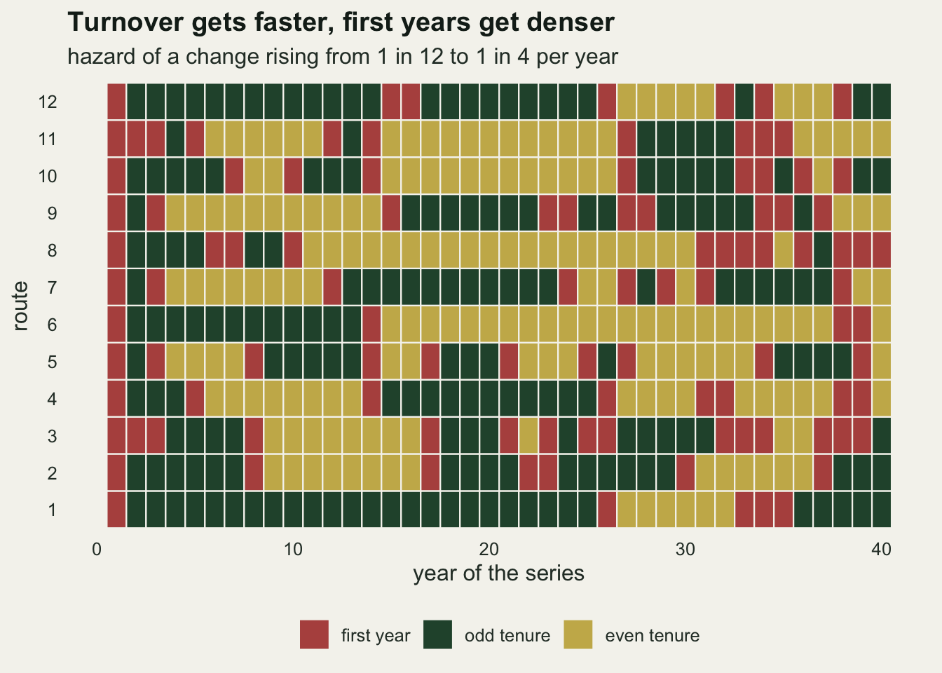
Three fits on the same counts
Three Poisson log-linear models are fitted with a fixed year slope. The route model has a factor for route and no observer information, which is what a route analysis looks like when observer identity was never recorded. The observer model replaces the route factor with a factor for observer on route; since each observer-on-route belongs to one route, the route means are absorbed. The first-year model adds a single 0/1 column that is one in each observer’s first year on the route, which is the covariate Kendall and colleagues tested and the start-up term in Link and Sauer’s hierarchical model. Overdispersion is handled with a quasi-Poisson scale, so the intervals use a Pearson dispersion estimate.
In glm() each model is one line. With a factor of two hundred or more levels, though, each fit builds and inverts a wide design matrix, and a grid of several thousand fits is slow on a small machine. The fixed effects do not have to be estimated to get the slope: for a Poisson model with a group factor, the group intercepts can be profiled out exactly, leaving a Newton iteration on one or two parameters. The function below does that and returns the same estimate, standard error and quasi-Poisson dispersion as glm().
fe_poisson <- function(count, xmat, group, n_iter = 30) {
  xmat <- as.matrix(xmat)
  grp  <- as.integer(factor(group))
  y_tot <- rowsum(count, grp)[, 1]
  b <- rep(0, ncol(xmat))
  for (it in seq_len(n_iter)) {
    w_exp   <- exp(drop(xmat %*% b))
    p_share <- w_exp / rowsum(w_exp, grp)[grp, 1]   # share of the group total
    mu_hat  <- y_tot[grp] * p_share
    x_cent  <- xmat - rowsum(p_share * xmat, grp)[grp, , drop = FALSE]
    score <- colSums(x_cent * (count - mu_hat))
    info  <- crossprod(x_cent * sqrt(mu_hat))
    step  <- solve(info, score)
    b <- b + step
    if (max(abs(step)) < 1e-10) break
  }
  n_par <- ncol(xmat) + length(y_tot)
  keep  <- mu_hat > 0
  phi <- sum((count[keep] - mu_hat[keep])^2 / mu_hat[keep]) / (length(count) - n_par)
  list(coef = b, se = sqrt(diag(solve(info)) * phi))
}

glm_route <- glm(count ~ route + year_c, family = quasipoisson, data = panel_accel)
glm_obs   <- glm(count ~ obs + year_c, family = quasipoisson, data = panel_accel)
glm_first <- glm(count ~ obs + first + year_c, family = quasipoisson, data = panel_accel)
fast_route <- fe_poisson(panel_accel$count, cbind(panel_accel$year_c), panel_accel$route)
fast_obs   <- fe_poisson(panel_accel$count, cbind(panel_accel$year_c), panel_accel$obs)
fast_first <- fe_poisson(panel_accel$count, cbind(panel_accel$first, panel_accel$year_c),
                         panel_accel$obs)

glm_tab  <- rbind(summary(glm_route)$coefficients["year_c", 1:2],
                  summary(glm_obs)$coefficients["year_c", 1:2],
                  summary(glm_first)$coefficients["year_c", 1:2])
fast_tab <- rbind(c(fast_route$coef, fast_route$se),
                  c(fast_obs$coef, fast_obs$se),
                  c(fast_first$coef[2], fast_first$se[2]))
max_gap <- max(abs(glm_tab - fast_tab))
first_glm <- coef(glm_first)["first"]
n_levels_obs <- nlevels(panel_accel$obs)
On the accelerating network shown above, with a true trend of zero and a first-year deficit of 10 per cent, the three glm() fits put the year slope at +0.11, +0.51 and +0.21 per cent per year (log scale times 100), with standard errors of 0.07, 0.18 and 0.18. The first-year coefficient in the last model was -0.102 against a true -0.105. The observer factor had 315 levels. The largest absolute difference between the glm() table and the profiled fits, over all six estimates and standard errors, was 1.79e-09. From here on the profiled function stands in for glm().
This one network does not show the pattern the rest of the post measures: its observer fit sits above the route fit, but its first-year fit sits below both. The slope standard errors of the observer models are larger than a tenth of a per cent per year, so a single network cannot separate a bias of a few tenths from noise. The next section repeats it.
The observer term turns a first-year dip into an increase
The grid crosses the two turnover schedules with first-year deficits of 0, 5, 10 and 20 per cent and two true trends, zero and a decline of one per cent per year on the log scale. Each of the 16 cells gets 200 simulated networks, and each network gets all three fits. For every fit the grid keeps the slope, whether its 95 per cent interval covered the truth, and one property of the design that the next section needs.
n_rep <- 200
deficits <- c(0, 0.05, 0.10, 0.20)
cells <- expand.grid(beta = c(0, -0.01), schedule = c("constant", "accelerating"),
                     deficit = deficits, stringsAsFactors = FALSE)
model_names <- c("route only", "observer", "observer + first year")

one_network <- function(hazard, deficit, beta) {
  pan <- sim_panel(hazard, deficit, beta)
  f_r <- fe_poisson(pan$count, cbind(pan$year_c), pan$route)
  f_o <- fe_poisson(pan$count, cbind(pan$year_c), pan$obs)
  f_f <- fe_poisson(pan$count, cbind(pan$first, pan$year_c), pan$obs)
  est <- c(f_r$coef, f_o$coef, f_f$coef[2])
  se  <- c(f_r$se, f_o$se, f_f$se[2])
  # within-observer and within-route OLS slope of the first-year indicator on year
  yo <- pan$year_c - ave(pan$year_c, pan$obs); fo <- pan$first - ave(pan$first, pan$obs)
  yr <- pan$year_c - ave(pan$year_c, pan$route); fr <- pan$first - ave(pan$first, pan$route)
  c(est, abs(est - beta) < qnorm(0.975) * se,
    sum(fo * yo) / sum(yo^2), sum(fr * yr) / sum(yr^2))
}

grid_rows <- vector("list", nrow(cells))
for (k in seq_len(nrow(cells))) {
  set.seed(7000 + k)
  hz <- if (cells$schedule[k] == "constant") hazard_const else hazard_accel
  reps <- replicate(n_rep, one_network(hz, cells$deficit[k], cells$beta[k]))
  grid_rows[[k]] <- data.frame(
    cells[rep(k, 3), ], model = factor(model_names, levels = model_names),
    bias = 100 * (rowMeans(reps[1:3, ]) - cells$beta[k]),
    bias_se = 100 * apply(reps[1:3, ], 1, sd) / sqrt(n_rep),
    coverage = rowMeans(reps[4:6, ]),
    slope_obs = mean(reps[7, ]), slope_route = mean(reps[8, ]),
    row.names = NULL)
}
grid_res <- do.call(rbind, grid_rows)

pick <- function(b, s, d, m, col) {
  grid_res[[col]][grid_res$beta == b & grid_res$schedule == s &
                  abs(grid_res$deficit - d) < 1e-9 & grid_res$model == m]
}
max_bias_se <- max(grid_res$bias_se)
route_abs_max <- max(abs(grid_res$bias[grid_res$model == "route only"]))
first_abs_max <- max(abs(grid_res$bias[grid_res$model == "observer + first year"]))
bias_df <- grid_res[grid_res$beta == 0, ]
bias_df$schedule <- factor(bias_df$schedule, levels = c("constant", "accelerating"),
labels = c("constant turnover", "accelerating turnover"))
bias_plot <- ggplot(bias_df, aes(100 * deficit, bias, colour = model)) +
geom_hline(yintercept = 0, colour = te_body, linewidth = 0.4, linetype = "dashed") +
geom_line(linewidth = 0.9) +
geom_point(size = 2.2) +
geom_errorbar(aes(ymin = bias - 2 * bias_se, ymax = bias + 2 * bias_se),
width = 0.8, linewidth = 0.5) +
facet_wrap(~ schedule) +
scale_colour_manual(values = c(te_gold, te_rust, te_forest), name = NULL) +
scale_x_continuous(breaks = 100 * deficits) +
labs(x = "first-year deficit (per cent)", y = "trend error (per cent per year)",
title = "The observer term manufactures an increase",
subtitle = "a stable population; three fits of the same counts") +
theme_datasheet() +
theme(legend.position = "bottom", strip.text = element_text(colour = te_ink))
bias_plot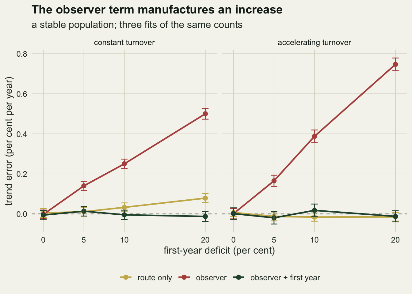
The route-only fit had a small bias, not a zero one: across all 16 cells its largest absolute mean error was 0.079 per cent per year, and the Monte Carlo standard error of any mean in the grid was at most 0.017. Under constant turnover it was pushed up, by +0.079 per cent per year (Monte Carlo standard error 0.011) in a stable population with a 20 per cent deficit, well beyond Monte Carlo noise. Accelerating turnover with the same deficit, the scenario built to produce a spurious decline, gave -0.014 (standard error 0.011). At these settings the intuitive decline is a few hundredths of a per cent per year at most; the next section shows why, and when it grows.
The observer fit is the one that goes wrong. With a 10 per cent deficit it reported a trend of +0.250 per cent per year under constant turnover and +0.388 under accelerating turnover; at a 20 per cent deficit the figures were +0.500 and +0.747. Turnover does not need to change for this to happen; a steady supply of novices is enough, and faster turnover makes it larger. Adding the first-year indicator brought every cell back: its largest mean error was 0.032 per cent per year.
The same pattern holds under a real decline. With the true trend at minus one per cent per year and a 10 per cent deficit, the observer fit was off by +0.244 and +0.378 per cent per year under the two schedules, so the decline it reports is shallower than the truth by about the amount it added to a stable population (slightly more under accelerating turnover). The first-year fit was off by -0.018 and -0.005.
Where the increase comes from
The route factor and the observer factor ask the data different questions. With a route factor, the slope compares years across a whole route; a first year can fall anywhere in the series, and what matters is only whether first years pile up early or late. With an observer factor, the slope is estimated from comparisons inside each tenure. Inside a tenure the first year is, by definition, the earliest year. A low first year followed by ordinary years looks, from inside the tenure, like a count that went up, and every tenure contributes the same small upward step.
That can be written down. Leaving a column out of a regression moves the fitted slope by the omitted coefficient times the slope of the omitted column on the included one, after both are adjusted for the other terms in the model. Here the omitted coefficient is log(1 - d), which is negative, and the auxiliary slope is the slope of the first-year indicator on year after centring both within observer. For a single tenure of L years, the indicator is one at the first year and zero after it, and its least squares slope on year is exactly -6 / (L (L + 1)). Pooled over tenures of different lengths it is -6 times the sum of (L - 1) divided by the sum of (L cubed - L). Both are negative, so the bias is positive. One-year tenures add nothing to either sum, and long tenures carry most of the variance in year, which is why the slope stays small but never zero.
seg_len_accel <- as.vector(table(panel_accel$obs))
closed_slope <- -6 * sum(seg_len_accel - 1) / sum(seg_len_accel^3 - seg_len_accel)
yo_one <- panel_accel$year_c - ave(panel_accel$year_c, panel_accel$obs)
fo_one <- panel_accel$first - ave(panel_accel$first, panel_accel$obs)
ols_slope <- sum(fo_one * yo_one) / sum(yo_one^2)
closed_gap <- abs(closed_slope - ols_slope)

mech_df <- grid_res[grid_res$model == "observer" & grid_res$deficit > 0, ]
mech_df$predicted <- 100 * log(1 - mech_df$deficit) * mech_df$slope_obs
mech_ratio <- mech_df$bias / mech_df$predicted
route_pred <- 100 * log(1 - 0.2) *
  grid_res$slope_route[grid_res$model == "route only" & grid_res$deficit == 0.2]
route_meas <- grid_res$bias[grid_res$model == "route only" & grid_res$deficit == 0.2]
late_rows <- panel_accel$year > 1
yr_late <- panel_accel$year_c[late_rows] - ave(panel_accel$year_c[late_rows], panel_accel$route[late_rows])
fr_late <- panel_accel$first[late_rows] - ave(panel_accel$first[late_rows], panel_accel$route[late_rows])
route_late_pred <- 100 * log(1 - 0.2) * sum(fr_late * yr_late) / sum(yr_late^2)
slope_obs_const <- pick(0, "constant", 0.1, "observer", "slope_obs")
slope_obs_accel <- pick(0, "accelerating", 0.1, "observer", "slope_obs")
On the accelerating network used earlier, the closed form gives an auxiliary slope of -0.03257, and the within-observer least squares slope computed from the data matches it exactly. Averaged over the grid’s networks, the auxiliary slope was -0.02462 under constant turnover and -0.03640 under accelerating turnover, and that difference carries most of the gap between the schedules.
Multiplying log(1 - d) by the mean auxiliary slope predicts the observer fit’s bias in each of the 12 cells with a nonzero deficit. The measured bias was between 0.88 and 1.10 times the prediction. The prediction is a least squares argument applied to a Poisson fit, which weights high counts more heavily and is not linear in the omitted term, so exact agreement is not expected; the sign and the ordering of the cells are carried by one design quantity.
The same calculation for the route factor explains why the intuitive worry stays small here. There the auxiliary slope is the slope of the first-year indicator on year within route. Leaving out year one, first years do become more common as the accelerating series goes on, and in the network shown earlier that part of the design alone predicts a trend error of -0.115 per cent per year at a 20 per cent deficit. But year one is a first year on every route, and that block of novices at the start pulls the slope the other way. With both parts in, the route-factor calculation predicts errors between -0.019 and +0.072 per cent per year at a 20 per cent deficit, and the route-only fit measured between -0.014 and +0.079.
That cancellation depends on the series starting when the routes do. A trend fitted over a window that starts later loses the block, and the check below refits the route-only model to years 11 to 40 of accelerating networks with a 20 per cent deficit and a stable population.
n_window <- 150
set.seed(7101)
window_slope <- replicate(n_window, {
  pan <- sim_panel(hazard_accel, deficit = 0.2, beta = 0)
  pan <- pan[pan$year > 10, ]
  pan$year_c <- pan$year - mean(pan$year)
  fe_poisson(pan$count, cbind(pan$year_c), pan$route)$coef
})
window_bias <- 100 * mean(window_slope)
window_mcse <- 100 * sd(window_slope) / sqrt(n_window)
Over 150 networks the windowed route-only trend was off by -0.068 per cent per year, with a Monte Carlo standard error of 0.018: the intuitive decline, sitting 3.7 standard errors from zero.
mech_df$schedule <- factor(mech_df$schedule, levels = c("constant", "accelerating"))
mech_df$true_trend <- ifelse(mech_df$beta == 0, "true trend 0", "true trend -1 per cent")
lim_top <- 1.08 * max(c(mech_df$predicted, mech_df$bias))
ggplot(mech_df, aes(predicted, bias)) +
  geom_abline(slope = 1, intercept = 0, colour = te_body, linetype = "dashed", linewidth = 0.4) +
  geom_errorbar(aes(ymin = bias - 2 * bias_se, ymax = bias + 2 * bias_se, colour = schedule),
                width = 0, linewidth = 0.5) +
  geom_point(aes(colour = schedule, shape = true_trend), size = 2.8) +
  scale_colour_manual(values = c(constant = te_forest, accelerating = te_rust), name = NULL) +
  scale_shape_manual(values = c(16, 1), name = NULL) +
  coord_equal(xlim = c(0, lim_top), ylim = c(0, lim_top)) +
  labs(x = "predicted: log(1 - d) times auxiliary slope", y = "measured bias (per cent per year)",
       title = "One design quantity carries the bias",
       subtitle = "dashed line: measured equals predicted") +
  theme_datasheet() +
  theme(legend.position = "right")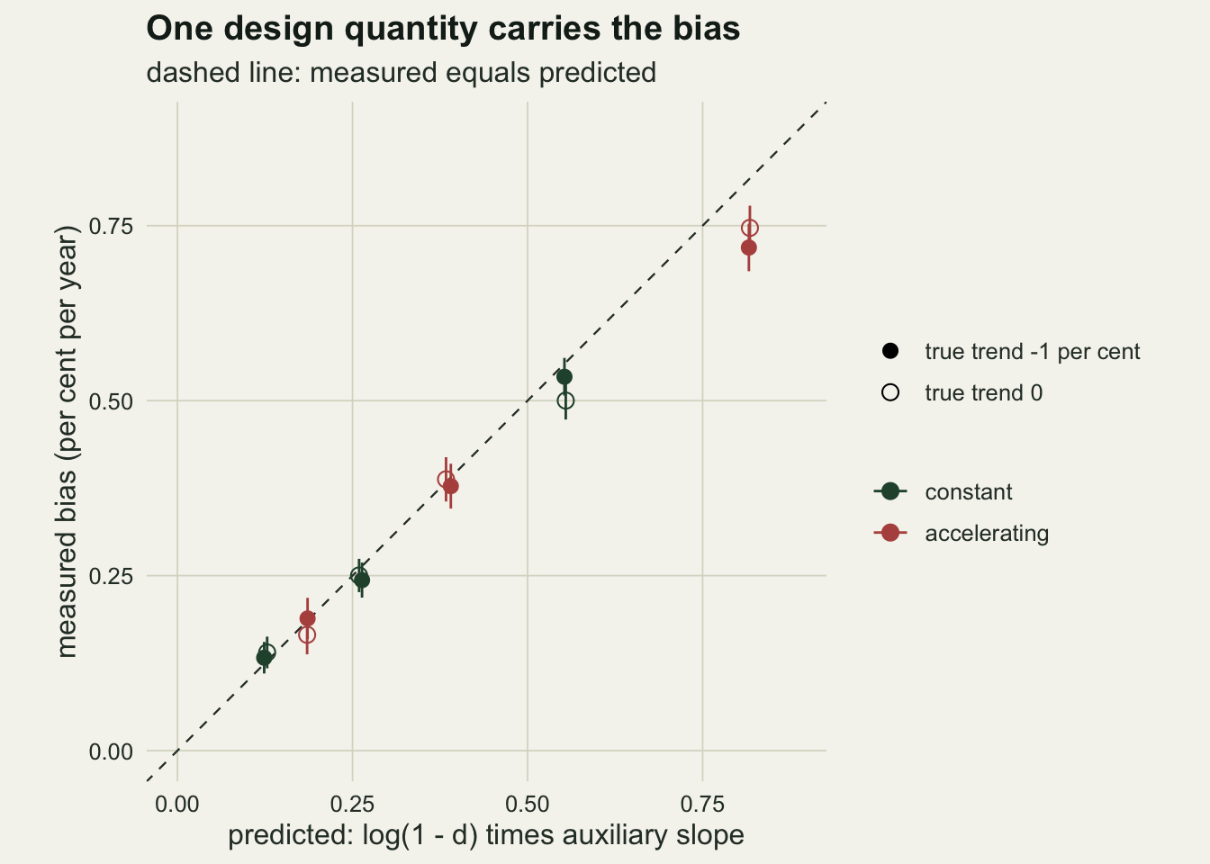
The fit without observers: small bias, overconfident
A route-only trend with a small bias (at most 0.08 per cent per year in the grid, from the all-novice first year) is not a reason to drop observer identity. Observers differ, and a route counted by a strong observer for nine years and then a weak one for eleven carries a step that the route factor cannot see. Each step is independent of year, so it does not bias the slope on average, but it makes the residuals within a route correlated for as long as a tenure lasts, and a quasi-Poisson dispersion treats every route-year as independent.
cov_route <- range(grid_res$coverage[grid_res$model == "route only"])
cov_obs_10 <- c(pick(-0.01, "constant", 0.1, "observer", "coverage"),
                pick(-0.01, "accelerating", 0.1, "observer", "coverage"))
cov_obs_20 <- c(pick(-0.01, "constant", 0.2, "observer", "coverage"),
                pick(-0.01, "accelerating", 0.2, "observer", "coverage"))
cov_first <- range(grid_res$coverage[grid_res$model == "observer + first year"])
cov_obs_0 <- range(grid_res$coverage[grid_res$model == "observer" & grid_res$deficit == 0])
cov_mcse <- sqrt(0.95 * 0.05 / n_rep)

# the same route-only fit with no observer variance at all
n_noobs <- 150
sd_obs_keep <- sd_obs
sd_obs <- 0
set.seed(7201)
noobs_reps <- replicate(n_noobs, one_network(hazard_const, deficit = 0.1, beta = -0.01))
sd_obs <- sd_obs_keep
cov_route_noobs <- mean(noobs_reps[4, ])
cov_noobs_mcse <- sqrt(cov_route_noobs * (1 - cov_route_noobs) / n_noobs)
cov_df <- grid_res[grid_res$beta == -0.01, ]
cov_df$schedule <- factor(cov_df$schedule, levels = c("constant", "accelerating"),
labels = c("constant turnover", "accelerating turnover"))
ggplot(cov_df, aes(100 * deficit, coverage, colour = model)) +
geom_hline(yintercept = 0.95, colour = te_body, linetype = "dashed", linewidth = 0.4) +
geom_line(linewidth = 0.9) +
geom_point(size = 2.2) +
facet_wrap(~ schedule) +
scale_colour_manual(values = c(te_gold, te_rust, te_forest), name = NULL) +
scale_x_continuous(breaks = 100 * deficits) +
scale_y_continuous(limits = c(0, 1)) +
labs(x = "first-year deficit (per cent)", y = "interval coverage",
title = "A small bias is not calibration",
subtitle = "dashed line: the nominal 95 per cent") +
theme_datasheet() +
theme(legend.position = "bottom", strip.text = element_text(colour = te_ink))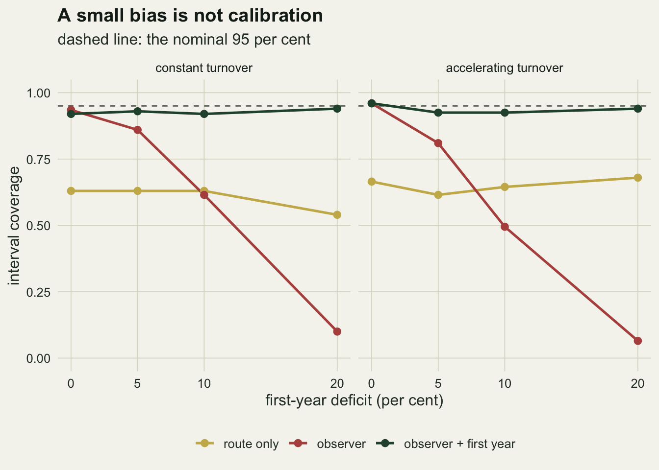
The route-only intervals covered the true trend in between 54 and 68 per cent of networks across the grid, whatever the deficit, against a nominal 95 and a Monte Carlo standard error of 1.5 percentage points for a rate near 95. That is mostly the cost of ignoring the observer steps: with no observer variance, constant turnover, a 10 per cent deficit and a real decline, the same fit covered 87 per cent of 150 networks (standard error 2.8 points), closer to nominal but not there.
The observer fit is calibrated when there is no first-year effect, with coverage between 94 and 96 per cent in the zero-deficit cells. Its intervals are sized for the noise and know nothing about the bias, so once the bias appears they miss: with a 10 per cent deficit and a real decline, coverage fell to 62 per cent under constant turnover and 50 under accelerating turnover, and at 20 per cent to 10 and 6. The first-year fit stayed between 92 and 97 per cent in every cell.
What to report
Say whether observer identity entered the trend model, and at what level: an observer factor, an observer-on-route factor, or none. These are different models and they give different answers from the same counts.
If observer effects are in the model, add a first-year indicator defined per observer on each route, or say why not. The indicator costs one degree of freedom. Without it the trend inherits log(1 - d) times the within-observer slope of the first-year indicator on year, and that slope can be computed from the observer table before any counts are modelled; the closed form above needs only the tenure lengths.
Report the first-year coefficient with its interval. It is the direct estimate of the novice deficit, and a scheme that sees a large one has a training question as well as a statistical one.
Report the tenure distribution of the network: observers per route, the share of single-year tenures, and whether the share of first years changes over the series. A reader cannot judge the size of either bias in this post without it.
If the model has no observer term, do not report its interval as though route-years were independent. When observer quality does not drift over the series and the trend window starts with the survey, the trend moves little there; the standard error is what goes wrong.
Honest limits
Observer quality here has no trend over the series: a new observer is drawn from the same distribution in year 35 as in year 2. In the Breeding Bird Survey it does drift, with later observers counting more (Sauer, Peterjohn and Link 1994), and that is a bias the route-only fit would carry on top of the small one measured here. An observer factor absorbs each observer’s level and should remove it, though that case was not simulated; it is the reason to keep observer identity and add the first-year indicator, not to drop both.
Every route here starts in year one with a new observer. The windowed check above shows that a trend over years 11 to 40 loses that block and the route-only fit then shows the intuitive decline; a real scheme whose routes join at different times sits somewhere between the two, and that mix was not simulated.
The observer effects here are fixed. The survey models in the references treat them as random, drawn from a distribution with an estimated variance, and a random effect shrinks short tenures towards the mean. Shrinkage borrows some of the between-tenure comparison that the route factor makes, so a random observer effect without a first-year term should sit somewhere between the route-only and the observer results measured here. Where it sits depends on the observer variance and the tenure lengths, and it was not measured: a mixed model fit on a few hundred observer levels is too slow to repeat thousands of times in this post.
The first-year deficit is a single step in year one and nothing after it. If learning is instead a curve over two or three seasons, every tenure carries a longer rise at its start, and one indicator would be expected to remove only part of the bias; that case was not simulated. The same auxiliary-slope argument applies, with the learning curve in place of the indicator.
The turnover schedules and variance components are design constants, fixed before any fitting, and the tenures are geometric: every observer is equally likely to leave in any year. There is no reason to expect real volunteer tenures to follow that shape, and a network with a different mix of short and long tenures has a different auxiliary slope. The closed form handles any set of tenure lengths, which is the reason to compute it from a real observer table rather than trust the numbers above.
Everything is a single species on routes of equal size and a linear trend on the log scale. Nothing here says how the bias moves with abundance: at low counts the Poisson weights differ and the first-year coefficient is estimated with much less precision, so a first-year model may need to share the indicator across species.
References
Sauer JR, Peterjohn BG, Link WA 1994 The Auk 111(1):50-62 (10.2307/4088504)
Kendall WL, Peterjohn BG, Sauer JR 1996 The Auk 113(4):823-829 (10.2307/4088860)
Link WA, Sauer JR 2002 Ecology 83(10):2832-2840 (10.1890/0012-9658(2002)083[2832:AHAOPC]2.0.CO;2)