---
title: "Variance components in monitoring data"
description: "Split monitoring data into site, year, interaction and residual variance in base R, and see why the largest component is free for trend and fatal for status."
date: "2026-06-26 09:00"
date-modified: "2026-10-01"
categories: [R, survey design, monitoring, ecology tutorial]
image: thumbnail.png
image-alt: "Bar chart of four variance components with their separate contributions to a status estimate and to a trend estimate"
---
*Corrected 1 October 2026: the comparison of the naive and two-stage trend intervals said their coverages came from the same data; they come from separate runs of the same simulation, and the sentence now says so.*
A monitoring programme visits a set of sites, counts something, and repeats for years. The numbers vary for four different reasons, and a programme that cannot tell them apart cannot say what its own data are good for.
Some sites are simply richer than others, and they stay that way. Some years are good everywhere at once, and some are bad everywhere at once. Some sites are good in a particular year for reasons local to that site. And two visits to the same site in the same season give different counts because counting is noisy.
Those four sources are the variance components. This post estimates them by hand from a balanced design, then shows the point that decides how a programme should be built: **the component that dominates one question contributes nothing at all to the other.**
## A model for monitoring data
Write the log count at site `i`, year `j`, visit `k` as a mean, a linear trend, and four random parts.
```{r setup-model}
# y_ijk = mu + beta*(t_j - tbar) + s_i + a_j + (sa)_ij + e_ijk
#   s_i   persistent differences between sites
#   a_j   a good year or a bad year, shared by every site
#   sa_ij site-by-year interaction: this site, this year
#   e_ijk within-season counting noise

sim_monitoring <- function(n_site, n_year, n_rep, beta,
                           sd_site, sd_year, sd_sy, sd_res, mu = 3) {
  s  <- rnorm(n_site, 0, sd_site)
  a  <- rnorm(n_year, 0, sd_year)
  sa <- matrix(rnorm(n_site * n_year, 0, sd_sy), n_site, n_year)
  t  <- seq_len(n_year)
  tc <- t - mean(t)
  d  <- expand.grid(rep = seq_len(n_rep), site = seq_len(n_site), year = seq_len(n_year))
  d$y <- mu + beta * tc[d$year] + s[d$site] + a[d$year] +
         sa[cbind(d$site, d$year)] + rnorm(nrow(d), 0, sd_res)
  d$site <- factor(d$site); d$yearf <- factor(d$year); d$t <- t[d$year]
  list(d = d, s = s, a = a)
}

sd_site <- 0.55   # among sites
sd_year <- 0.20   # among years, shared
sd_sy   <- 0.30   # site by year
sd_res  <- 0.35   # repeat visits
beta_true <- -0.03            # about 3 per cent per year on the log scale
n_site <- 30; n_year <- 10; n_rep <- 2

set.seed(367)
demo <- sim_monitoring(n_site, n_year, n_rep, beta_true, sd_site, sd_year, sd_sy, sd_res)
dd <- demo$d   # the simulated data set used in the rest of the post

v_true <- c(site = sd_site^2, year = sd_year^2, sy = sd_sy^2, res = sd_res^2)
v_tot  <- sum(v_true)
data.frame(component = c("site", "year", "site by year", "repeat visit"),
           variance  = round(unname(v_true), 4),
           per_cent  = round(100 * unname(v_true) / v_tot, 1))
```
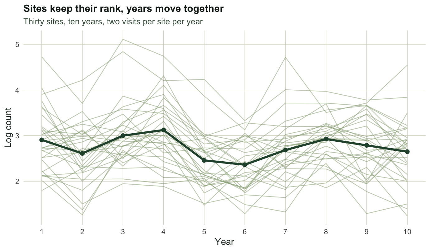
The site component is the largest by a wide margin, at `r sprintf("%.1f", 100 * v_true["site"] / v_tot)` per cent of the total. The year component is the smallest of the structured parts, at `r sprintf("%.1f", 100 * v_true["year"] / v_tot)` per cent. Hold on to that ordering, because it reverses later.
```{r fig-data}
#| echo: false
#| fig-width: 7.2
#| fig-height: 4.2
#| fig-cap: "Ten years of simulated monitoring data. Grey lines are individual sites, which cross one another often; the dark line is the annual mean across all 30 sites. The wobble in the dark line is the year component, and it is the same wobble for every site."
#| fig-alt: "Line chart with thirty faint grey site trajectories spread vertically and one dark green annual mean line running through the middle with a mild downward slope."
library(ggplot2)
theme_te <- function(base_size = 11) {
theme_minimal(base_size = base_size) +
theme(plot.background = element_rect(fill = "#f5f4ee", colour = NA),
panel.background = element_rect(fill = "#f5f4ee", colour = NA),
panel.grid.minor = element_blank(),
panel.grid.major = element_line(colour = "#dad9ca", linewidth = 0.3),
text = element_text(colour = "#2c3a31"),
plot.title = element_text(colour = "#16241d", face = "bold", size = base_size + 1),
plot.subtitle = element_text(colour = "#46604a", size = base_size - 1),
plot.caption = element_text(colour = "#5d6b61", size = base_size - 2))
}
site_year <- aggregate(y ~ site + t, data = dd, FUN = mean)
ann <- aggregate(y ~ t, data = dd, FUN = mean)
ggplot(site_year, aes(t, y)) +
geom_line(aes(group = site), colour = "#93a87f", alpha = 0.55, linewidth = 0.4) +
geom_line(data = ann, colour = "#275139", linewidth = 1.2) +
geom_point(data = ann, colour = "#275139", size = 2) +
scale_x_continuous(breaks = 1:10) +
labs(x = "Year", y = "Log count",
title = "Years move together",
subtitle = "Thirty sites, ten years, two visits per site per year") +
theme_te()
```
## Splitting the variance by hand
The design is balanced, so the four components come straight out of the two-way analysis of variance. Each mean square has a known expectation, and inverting those expectations gives moment estimators. No mixed-model package is needed.
```{r vc-estimator}
vc_anova <- function(d, n_site, n_year, n_rep, detrended = FALSE) {
  y <- d$y; gm <- mean(y)
  m_si   <- tapply(y, d$site, mean)
  m_yr   <- tapply(y, d$yearf, mean)
  m_cell <- tapply(y, list(d$site, d$yearf), mean)

  SS_site <- n_year * n_rep * sum((m_si - gm)^2)
  SS_year <- n_site * n_rep * sum((m_yr - gm)^2)
  SS_sy   <- n_rep * sum((m_cell - outer(m_si, m_yr, "+") + gm)^2)
  SS_res  <- sum((y - m_cell[cbind(as.integer(d$site), as.integer(d$yearf))])^2)

  # removing a linear trend first costs one year degree of freedom
  df_year <- if (detrended) n_year - 2 else n_year - 1
  MS_site <- SS_site / (n_site - 1)
  MS_year <- SS_year / df_year
  MS_sy   <- SS_sy   / ((n_site - 1) * (n_year - 1))
  MS_res  <- SS_res  / (n_site * n_year * (n_rep - 1))

  c(site = (MS_site - MS_sy) / (n_rep * n_year),
    year = (MS_year - MS_sy) / (n_rep * n_site),
    sy   = (MS_sy - MS_res) / n_rep,
    res  = MS_res)
}

dd$y_detr <- residuals(lm(y ~ t, data = dd))   # take the trend out first
d_detr <- dd; d_detr$y <- dd$y_detr
v_hat <- vc_anova(d_detr, n_site, n_year, n_rep, detrended = TRUE)
round(rbind(estimate = v_hat, truth = v_true), 4)
```
One data set gives `r sprintf("%.3f", v_hat["site"])` for the site component against a true `r sprintf("%.3f", v_true["site"])`, and `r sprintf("%.3f", v_hat["year"])` for the year component against `r sprintf("%.3f", v_true["year"])`. Over repeated data sets the estimator sits on the truth.
```{r vc-mc}
set.seed(3671)
B <- 400
vc_reps <- t(replicate(B, {
  z <- sim_monitoring(n_site, n_year, n_rep, beta_true, sd_site, sd_year, sd_sy, sd_res)$d
  z$y <- residuals(lm(y ~ t, data = z))
  vc_anova(z, n_site, n_year, n_rep, detrended = TRUE)
}))
vc_mean <- colMeans(vc_reps)
vc_sd   <- apply(vc_reps, 2, sd)
round(rbind(mean = vc_mean, truth = v_true, sd = vc_sd), 4)
```
The detrending step matters. A linear trend lives entirely in the year means, so if it is left in, it is counted as year-to-year variance. Removing it costs one degree of freedom among the years, and the estimator has to be told.
Notice the last row. The site component is estimated with a standard deviation of `r sprintf("%.3f", vc_sd["site"])` from 30 sites, and the year component with `r sprintf("%.3f", vc_sd["year"])` from 10 years. Ten years is a small sample of years, and that shows up again in the checking post of this series.
## The same variance, two different questions
A monitoring programme is usually asked two questions. What is the state of the region now, and is it changing? The two use the same data and the same components, but not in the same way.
**Status.** The estimate for one year is the mean over the sampled sites. The year effect for that year is part of what happened, not part of the error, so the error variance is the site, interaction and residual parts divided by the number of sites.
**Trend.** With the same sites revisited every year, each site's persistent level is common to all its years, so it shifts the whole trajectory up or down and leaves the slope alone. It drops out completely. The year effect does not drop out: a good year early and a bad year late is a downward slope with no population change behind it.
```{r estimands}
Sxx <- n_year * (n_year^2 - 1) / 12          # sum of squares of centred year index

var_status <- (v_true["site"] + v_true["sy"] + v_true["res"] / n_rep) / n_site
var_trend  <- (v_true["year"] + (v_true["sy"] + v_true["res"] / n_rep) / n_site) / Sxx

share_status <- 100 * v_true["site"] / (v_true["site"] + v_true["sy"] + v_true["res"] / n_rep)
share_trend  <- 100 * v_true["year"] / (v_true["year"] + (v_true["sy"] + v_true["res"] / n_rep) / n_site)

round(c(se_status = sqrt(unname(var_status)), se_trend = sqrt(unname(var_trend)),
        site_pct_of_status = unname(share_status),
        year_pct_of_trend  = unname(share_trend)), 4)
```
```{r estimand-mc}
set.seed(3672)
B <- 1500
mc <- t(replicate(B, {
  z <- sim_monitoring(n_site, n_year, n_rep, beta_true, sd_site, sd_year, sd_sy, sd_res)
  am <- tapply(z$d$y, z$d$yearf, mean)
  truth_y1 <- 3 + beta_true * (1 - mean(seq_len(n_year))) + z$a[1]
  c(status_err = unname(am[1]) - truth_y1,
    slope = unname(coef(lm(am ~ seq_len(n_year)))[2]))
}))
round(c(sd_status_mc = sd(mc[, "status_err"]), sd_status_formula = sqrt(unname(var_status)),
        sd_slope_mc = sd(mc[, "slope"]), sd_slope_formula = sqrt(unname(var_trend)),
        mean_slope  = mean(mc[, "slope"])), 5)
```
Simulation agrees with the formulas: `r sprintf("%.4f", sd(mc[, "status_err"]))` against `r sprintf("%.4f", sqrt(var_status))` for status, and `r sprintf("%.5f", sd(mc[, "slope"]))` against `r sprintf("%.5f", sqrt(var_trend))` for the trend. Now compare the two decompositions.
```{r fig-shares}
#| echo: false
#| fig-width: 7.2
#| fig-height: 4.4
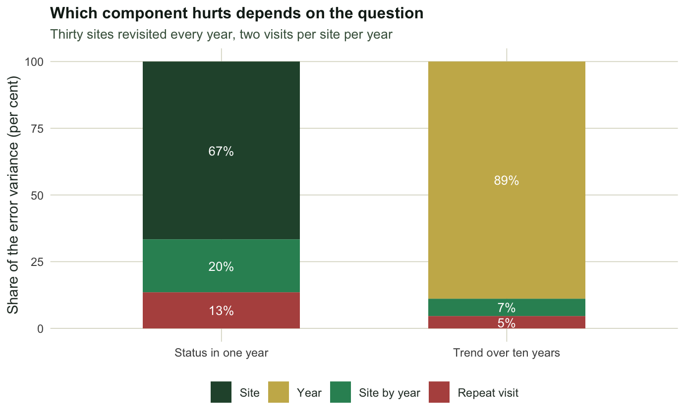
#| fig-cap: "The same four components, weighted twice. On the left, the share each one contributes to the error of a single-year status estimate. On the right, the share it contributes to the error of the trend. The site component is two thirds of the first bar and exactly zero in the second; the year component is zero in the first and most of the second."
#| fig-alt: "Two stacked bars side by side. The status bar is dominated by the site component in dark green; the trend bar is dominated by the year component in gold, with no site segment at all."
w_status <- c(site = unname(v_true["site"]), year = 0,
sy = unname(v_true["sy"]), res = unname(v_true["res"]) / n_rep) / n_site
w_trend <- c(site = 0, year = unname(v_true["year"]),
sy = unname(v_true["sy"]) / n_site, res = unname(v_true["res"]) / n_rep / n_site) / Sxx
shares <- data.frame(
question = rep(c("Status in one year", "Trend over ten years"), each = 4),
component = rep(c("Site", "Year", "Site by year", "Repeat visit"), 2),
pct = c(100 * w_status / sum(w_status), 100 * w_trend / sum(w_trend)))
shares$component <- factor(shares$component,
levels = c("Site", "Year", "Site by year", "Repeat visit"))
ggplot(shares, aes(question, pct, fill = component)) +
geom_col(width = 0.55) +
geom_text(aes(label = ifelse(pct > 4, sprintf("%.0f%%", pct), "")),
position = position_stack(vjust = 0.5), colour = "white", size = 3.4) +
scale_fill_manual(values = c(Site = "#275139", Year = "#c9b458",
`Site by year` = "#2f8f63", `Repeat visit` = "#b5534e")) +
labs(x = NULL, y = "Share of the error variance (per cent)", fill = NULL,
title = "Which component hurts depends on the question",
subtitle = "Thirty sites revisited every year, two visits per site per year") +
theme_te() + theme(legend.position = "bottom")
```
The site component is `r sprintf("%.1f", share_status)` per cent of the status error and nothing at all in the trend. The year component is `r sprintf("%.1f", 100 * v_true["year"] / v_tot)` per cent of the raw variance in the data and `r sprintf("%.1f", share_trend)` per cent of the trend error. The smallest structured component is the one that decides whether a trend can be seen.
There is a second consequence, and it is the harder one. Adding sites divides the site, interaction and residual parts by a larger number, but it does not touch the year part at all. **No number of sites reduces the year component.** That sets a floor on trend precision which only more years can lower.
## What this does to a naive analysis
The obvious regression fits every observation, absorbs the site differences as fixed effects, and reads off the year coefficient. The point estimate is fine. The standard error is not, because the year effect makes all sites in the same year move together, and a regression that assumes independent residuals cannot know that.
```{r naive-se}
set.seed(3673)
B <- 500
naive <- t(replicate(B, {
  z  <- sim_monitoring(n_site, n_year, n_rep, beta_true, sd_site, sd_year, sd_sy, sd_res)$d
  f  <- lm(y ~ t + site, data = z)
  co <- summary(f)$coefficients["t", ]
  ci <- unname(co[1]) + c(-1, 1) * qt(0.975, f$df.residual) * unname(co[2])
  c(est = unname(co[1]), se = unname(co[2]),
    covered = as.numeric(ci[1] <= beta_true && beta_true <= ci[2]))
}))
naive_se   <- mean(naive[, "se"])
naive_sd   <- sd(naive[, "est"])
naive_cov  <- mean(naive[, "covered"])
round(c(reported_se = naive_se, true_sd = naive_sd,
        ratio = naive_sd / naive_se, coverage = naive_cov), 4)
```
The regression reports a standard error of `r sprintf("%.4f", naive_se)` when the estimate actually varies with a standard deviation of `r sprintf("%.4f", naive_sd)`, a factor of `r sprintf("%.2f", naive_sd / naive_se)`. Its nominal 95 per cent interval contains the true trend `r sprintf("%.0f", 100 * naive_cov)` per cent of the time.
The two-stage estimator used above avoids this. Average within each year first, then regress the `r n_year` annual means on year. The annual mean carries the year effect as a single number, so the regression sees the right amount of noise, and the interval behaves.
```{r two-stage-coverage}
set.seed(3674)
B <- 500
cov2 <- mean(replicate(B, {
  z  <- sim_monitoring(n_site, n_year, n_rep, beta_true, sd_site, sd_year, sd_sy, sd_res)$d
  am <- tapply(z$y, z$yearf, mean)
  f  <- lm(am ~ seq_len(n_year))
  ci <- confint(f)[2, ]
  as.numeric(ci[1] <= beta_true && beta_true <= ci[2])
}))
c(two_stage_coverage = cov2, naive_coverage = naive_cov)
```
Coverage `r sprintf("%.3f", cov2)` against `r sprintf("%.3f", naive_cov)`, from separate runs of the same simulation; on any one data set the two point estimates are identical, because the design is balanced. The difference is entirely in which components the analysis believes are there.
The honest limit of this post is that the split assumes the four components are constant over the period, and that the design is balanced. Unbalanced data are usually handled with a likelihood method such as REML rather than with these simple mean squares, and a component that itself changes over time (a monitoring scheme that quietly gets better at counting) is not in this model at all. That last one is the third check in the closing post of this series.
## Where this leaves the series
The variance components are not a summary statistic. They are the input to every design decision that follows: which sites to revisit, how many years to plan for, and what the programme can honestly promise to detect. The next post spends the same budget four different ways and measures what each one buys.
## References
Urquhart NS, Paulsen SG, Larsen DP 1998 Ecological Applications 8(2):246-257 (10.1890/1051-0761(1998)008[0246:MFPRRO]2.0.CO;2)
Larsen DP, Kincaid TM, Jacobs SE, Urquhart NS 2001 BioScience 51(12):1069-1078 (10.1641/0006-3568(2001)051[1069:DFELAR]2.0.CO;2)
Urquhart NS, Kincaid TM 1999 Journal of Agricultural, Biological, and Environmental Statistics 4(4):404-414 (10.2307/1400498)
Searle SR, Casella G, McCulloch CE 1992 Variance Components. Wiley, New York. ISBN 978-0-471-62162-1
## Related tutorials
- [Revisit designs for long-term monitoring](../revisit-designs-for-monitoring/)
- [Nested and crossed random effects in lme4](../nested-and-crossed-random-effects/)
- [Overdispersion, year noise and a wiggly GAM trend](../overdispersion-and-a-wiggly-trend/)
- [Random effects with too few levels](../random-effects-with-too-few-levels/)