---
title: "Nested and crossed random effects in lme4"
description: "Plots numbered one to four inside every site make lme4 fit four plots, not forty eight. Here is what the wrong formula does to the variance components."
date: "2026-08-08 12:00"
categories: [R, mixed models, experimental design, lme4, ecology tutorial]
image: thumbnail.png
image-alt: "Bar chart of estimated standard deviations for the plot and residual terms on a warm off-white panel. The wrong formula keeps barely a quarter of the true value in the plot term and inflates the residual, while the right formula lands close to the true values marked by diamonds."
---
The design lives in the formula. A mixed model has no idea which of your grouping columns are nested inside which, and it will not warn you if you get it wrong, because both readings are legitimate models. It simply fits the one you wrote.
The most common way to get it wrong is also the most invisible. Plots are numbered one to four inside every site, because that is how the field sheets were printed, so the column contains the numbers one to four and nothing else. Write `(1 | site) + (1 | plot)` and lme4 fits four plots for the whole study: plot one in Bialowieza and plot one in the Cairngorms are the same random effect. The model converges, the summary looks ordinary, and the plot variance comes out near zero.
This post fits both versions to data with known variance components, measures what the mistake costs, and then does the mirror image: data that really is crossed, fitted with a nested formula.
## Twelve sites, four plots each, five measurements per plot
```{r setup}
#| message: false
#| warning: false
library(ggplot2)
library(lme4)

te_paper  <- "#f5f4ee"
te_ink    <- "#16241d"
te_body   <- "#2c3a31"
te_forest <- "#275139"
te_rust   <- "#b5534e"
te_gold   <- "#c9b458"
te_line   <- "#dad9ca"

theme_datasheet <- function() {
  theme_minimal(base_size = 12) +
    theme(plot.background  = element_rect(fill = te_paper, colour = NA),
          panel.background = element_rect(fill = te_paper, colour = NA),
          panel.grid.major = element_line(colour = te_line, linewidth = 0.3),
          panel.grid.minor = element_blank(),
          text             = element_text(colour = te_body),
          plot.title       = element_text(colour = te_ink, face = "bold"),
          axis.text        = element_text(colour = te_body))
}
fit_ctl <- lmerControl(optimizer = "bobyqa")

n_site <- 12; n_plot <- 4; n_obs <- 5
sd_site <- 1.2; sd_plot <- 0.9; sd_res <- 0.7

simulate_nested <- function() {
  site  <- rep(seq_len(n_site), each = n_plot * n_obs)
  pnum  <- rep(rep(seq_len(n_plot), each = n_obs), n_site)  # 1 to 4 in every site
  pid   <- paste(site, pnum, sep = "_")
  fert  <- rep(rep(c(0, 0, 1, 1), each = n_obs), n_site)    # applied whole plots
  y <- 10 +
    rnorm(n_site, 0, sd_site)[site] +
    rnorm(n_site * n_plot, 0, sd_plot)[as.integer(factor(pid))] +
    rnorm(length(site), 0, sd_res)
  data.frame(y, fert, site = factor(site), pnum = factor(pnum),
             pid = factor(pid))
}
set.seed(7)
field <- simulate_nested()
head(field[c(1, 6, 21, 26), ], 4)
```
Site standard deviation `r sprintf("%.1f", sd_site)`, plot standard deviation `r sprintf("%.1f", sd_plot)`, residual `r sprintf("%.1f", sd_res)`, and the fertiliser treatment has no effect at all. Every plot in the study has its own random deviation, so there are `r sprintf("%d", n_site * n_plot)` plots, not `r sprintf("%d", n_plot)`.
## Two formulas, three variance components
```{r fits}
wrong <- lmer(y ~ fert + (1 | site) + (1 | pnum), field, control = fit_ctl)
right <- lmer(y ~ fert + (1 | site / pnum), field, control = fit_ctl)

sd_table <- function(m) {
  v <- as.data.frame(VarCorr(m))
  setNames(round(v$sdcor, 3), v$grp)
}
sd_table(wrong)
sd_table(right)
ngrps(wrong)
ngrps(right)
```
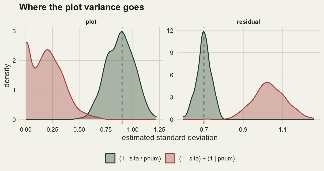
The wrong formula puts `r sprintf("%.2f", sd_table(wrong)[["pnum"]])` in the plot term and `r sprintf("%.2f", sd_table(wrong)[["Residual"]])` in the residual. The right one puts `r sprintf("%.2f", sd_table(right)[["pnum:site"]])` and `r sprintf("%.2f", sd_table(right)[["Residual"]])`, against true values of `r sprintf("%.1f", sd_plot)` and `r sprintf("%.1f", sd_res)`. A single study of this size does not pin the plot term down to two decimals, but it puts it somewhere rather than at zero. The plot to plot variation did not disappear under the wrong formula; it moved into the residual, where it looks like measurement noise.
The line that tells you which model you fitted is `ngrps()`. It reports `r sprintf("%d", ngrps(wrong)[["pnum"]])` plot groups for the wrong formula and `r sprintf("%d", ngrps(right)[["pnum:site"]])` for the right one. Anyone who knows the design knows which of those two numbers is correct, and it takes one line to look.
Three spellings give the correct fit, and they are the same model:
```{r spellings}
alt_a <- lmer(y ~ fert + (1 | site) + (1 | site:pnum), field, control = fit_ctl)
alt_b <- lmer(y ~ fert + (1 | site) + (1 | pid), field, control = fit_ctl)
c(nested_slash = logLik(right), explicit_interaction = logLik(alt_a),
  unique_labels = logLik(alt_b))
```
The third is the one to prefer in practice. Build a unique plot identifier when the data are read in, and the formula can no longer be ambiguous no matter who writes it.
## What the mistake costs
The fertiliser treatment in this simulation does nothing, and it is applied to whole plots, so it is the quantity most exposed to getting the plot term wrong.
```{r sweep}
#| warning: false
set.seed(1234)
n_sim <- 400
runs <- replicate(n_sim, {
  d  <- simulate_nested()
  fw <- lmer(y ~ fert + (1 | site) + (1 | pnum), d, control = fit_ctl)
  fr <- lmer(y ~ fert + (1 | site / pnum), d, control = fit_ctl)
  cw <- summary(fw)$coefficients[2, ]; cr <- summary(fr)$coefficients[2, ]
  vw <- as.data.frame(VarCorr(fw));    vr <- as.data.frame(VarCorr(fr))
  c(plot_w = vw$sdcor[vw$grp == "pnum"],  plot_r = vr$sdcor[vr$grp == "pnum:site"],
    res_w  = vw$sdcor[vw$grp == "Residual"], res_r = vr$sdcor[vr$grp == "Residual"],
    est_w  = cw[1], est_r = cr[1], se_w = cw[2], se_r = cr[2])
})
runs <- as.data.frame(t(runs))
names(runs) <- c("plot_w", "plot_r", "res_w", "res_r",
                 "est_w", "est_r", "se_w", "se_r")

cover_w <- mean(abs(runs$est_w) <= 1.96 * runs$se_w)
cover_r <- mean(abs(runs$est_r) <= 1.96 * runs$se_r)
se_ratio <- median(runs$se_r) / median(runs$se_w)
```
Over `r sprintf("%d", n_sim)` simulated studies the wrong formula estimates the plot standard deviation at a median of `r sprintf("%.2f", median(runs$plot_w))` against a true `r sprintf("%.1f", sd_plot)`, and the residual at `r sprintf("%.2f", median(runs$res_w))` against a true `r sprintf("%.1f", sd_res)`. The right formula gives `r sprintf("%.2f", median(runs$plot_r))` and `r sprintf("%.2f", median(runs$res_r))`.
The standard error of the treatment effect is `r sprintf("%.0f", 100 * (se_ratio - 1))` per cent larger under the right formula than under the wrong one, and a nominal 95 per cent interval covers the true value of zero `r sprintf("%.1f", 100 * cover_w)` per cent of the time instead of `r sprintf("%.1f", 100 * cover_r)`. The interval is not wrong by an order of magnitude. It is wrong by about the amount that turns a comfortable result into a significant one.
```{r fig-vc}
#| fig-cap: "Estimated standard deviations from 400 simulated studies for the plot and residual terms, under the two formulas. The dashed lines are the values the data were generated with."
#| fig-alt: "Two panels of density curves. In the plot term panel the wrong formula piles up near zero while the right formula sits on the dashed line at 0.9. In the residual panel the wrong formula sits well to the right of the dashed line at 0.7 and the right formula sits on it."
#| fig-width: 7.2
#| fig-height: 3.8
d_vc <- rbind(
  data.frame(sdv = runs$plot_w, term = "plot", formula = "(1 | site) + (1 | pnum)"),
  data.frame(sdv = runs$plot_r, term = "plot", formula = "(1 | site / pnum)"),
  data.frame(sdv = runs$res_w,  term = "residual", formula = "(1 | site) + (1 | pnum)"),
  data.frame(sdv = runs$res_r,  term = "residual", formula = "(1 | site / pnum)"))
truth <- data.frame(term = c("plot", "residual"), value = c(sd_plot, sd_res))

ggplot(d_vc, aes(sdv, fill = formula, colour = formula)) +
  geom_density(alpha = 0.35, linewidth = 0.7) +
  geom_vline(data = truth, aes(xintercept = value), colour = te_ink,
             linetype = "dashed", linewidth = 0.6) +
  facet_wrap(~ term, scales = "free") +
  scale_fill_manual(values = c("(1 | site) + (1 | pnum)" = te_rust,
                               "(1 | site / pnum)" = te_forest), name = NULL) +
  scale_colour_manual(values = c("(1 | site) + (1 | pnum)" = te_rust,
                                 "(1 | site / pnum)" = te_forest), name = NULL) +
  labs(x = "estimated standard deviation", y = "density",
       title = "Where the plot variance goes") +
  theme_datasheet() +
  theme(legend.position = "bottom",
        strip.text = element_text(colour = te_ink, face = "bold"))
```
## The mirror image: crossed data, nested formula
Sites visited every year for eight years, with several measurements per site per year. Year is not nested inside site: the same eight years apply to every site, and a wet year is wet everywhere. That is a crossed design, and the formula for it is `(1 | site) + (1 | year)`.
```{r crossed}
n_year <- 8; n_rep <- 3; sd_year <- 0.8

simulate_crossed <- function() {
  site <- rep(seq_len(n_site), each = n_year * n_rep)
  yr   <- rep(rep(seq_len(n_year), each = n_rep), n_site)
  y <- 10 + rnorm(n_site, 0, sd_site)[site] + rnorm(n_year, 0, sd_year)[yr] +
    rnorm(length(site), 0, sd_res)
  data.frame(y, site = factor(site), year = factor(yr))
}
set.seed(99)
survey <- simulate_crossed()

crossed <- lmer(y ~ (1 | site) + (1 | year), survey, control = fit_ctl)
nested  <- lmer(y ~ (1 | site / year), survey, control = fit_ctl)
sd_table(crossed)
sd_table(nested)
ngrps(nested)
```
The nested formula fits. It reports `r sprintf("%d", ngrps(nested)[["year:site"]])` groups for a term it calls `year:site`, and no year term at all, because `(1 | site / year)` expands to a site effect plus a site by year interaction and contains no main effect of year. The variance that belongs to years shared across all sites has been relabelled as variation between sites in their year to year behaviour.
That relabelling is a substantive claim. A shared year effect says the sites move together, driven by something regional such as weather. A site by year interaction says they do not. The two are opposite conclusions about synchrony, and the formula chose between them silently.
```{r crossed-sweep}
#| warning: false
set.seed(515)
n_sim2 <- 200
cross_runs <- as.data.frame(t(replicate(n_sim2, {
  d <- simulate_crossed()
  a <- lmer(y ~ (1 | site) + (1 | year), d, control = fit_ctl)
  b <- lmer(y ~ (1 | site / year), d, control = fit_ctl)
  va <- as.data.frame(VarCorr(a)); vb <- as.data.frame(VarCorr(b))
  c(year_ok = va$sdcor[va$grp == "year"],
    inter_bad = vb$sdcor[vb$grp == "year:site"],
    site_ok = va$sdcor[va$grp == "site"], site_bad = vb$sdcor[vb$grp == "site"])
})))
```
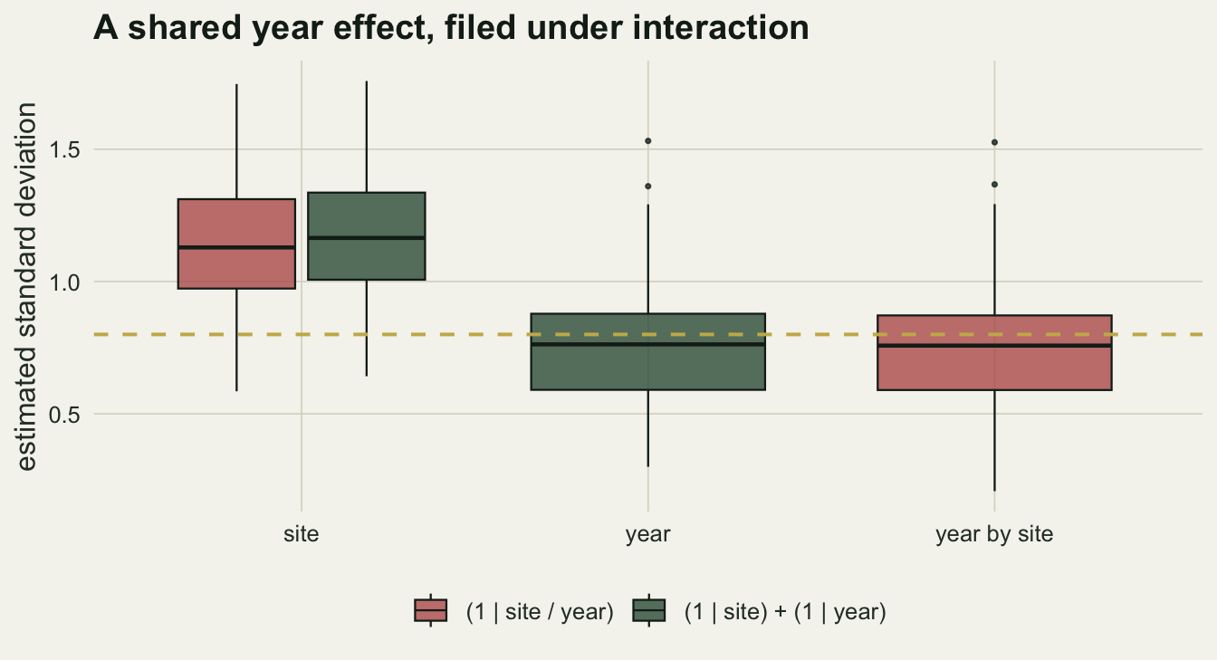
Across `r sprintf("%d", n_sim2)` simulated surveys with no site by year interaction whatsoever, the nested formula reports an interaction standard deviation of `r sprintf("%.2f", median(cross_runs$inter_bad))`. That is the same figure the crossed formula assigns to years, `r sprintf("%.2f", median(cross_runs$year_ok))`, against a true year standard deviation of `r sprintf("%.1f", sd_year)`. The year variance has not gone anywhere; it has been given a different name. The crossed formula leaves the site term at `r sprintf("%.2f", median(cross_runs$site_ok))` against a true `r sprintf("%.1f", sd_site)`.
```{r fig-crossed}
#| fig-cap: "Variance components from 200 simulated crossed surveys generated with no site by year interaction, under the crossed and the nested formula."
#| fig-alt: "Boxplots of estimated standard deviations. The crossed formula returns a year term near 0.8 and a site term near 1.2. The nested formula returns no year term, an interaction term near 0.8, and a site term slightly lower than the crossed one."
#| fig-width: 7
#| fig-height: 3.8
d_cr <- rbind(
  data.frame(sdv = cross_runs$year_ok,   term = "year",         who = "(1 | site) + (1 | year)"),
  data.frame(sdv = cross_runs$site_ok,   term = "site",         who = "(1 | site) + (1 | year)"),
  data.frame(sdv = cross_runs$inter_bad, term = "year by site", who = "(1 | site / year)"),
  data.frame(sdv = cross_runs$site_bad,  term = "site",         who = "(1 | site / year)"))

ggplot(d_cr, aes(term, sdv, fill = who)) +
  geom_boxplot(outlier.size = 0.6, linewidth = 0.4, colour = te_ink, alpha = 0.75) +
  geom_hline(yintercept = sd_year, colour = te_gold, linetype = "dashed",
             linewidth = 0.7) +
  scale_fill_manual(values = c("(1 | site) + (1 | year)" = te_forest,
                               "(1 | site / year)" = te_rust), name = NULL) +
  labs(x = NULL, y = "estimated standard deviation",
       title = "A shared year effect, filed under interaction") +
  theme_datasheet() +
  theme(legend.position = "bottom")
```
## What to report
Give the number of levels of every grouping factor. It is the output of one function, it takes a line in the methods, and it is the only thing in a mixed model summary that a reader can check against the design.
Build unique identifiers when the data are read in rather than at modelling time. A column of site and plot pasted together removes the entire class of error described here, and it costs one line.
State which grouping factors are crossed and which are nested, in words, next to the formula. Readers cannot infer it from the formula alone unless they already know the design, and neither can software.
Watch for a variance component reported as zero or nearly zero when the design says it should not be. That is the signature of the mistake, and it is much more often a labelling problem than a biological finding.
## Honest limits
Everything here is balanced: every site has four plots, every plot has five measurements, every site was visited in all eight years. Unbalanced designs behave less predictably, and the direction of the bias in the fixed effect standard error can go either way when the imbalance is related to the grouping structure.
The models are Gaussian with random intercepts only. Random slopes add a correlation parameter to every term and change the arithmetic, though not the labelling problem, which is upstream of any of that. Generalised linear mixed models add the further difficulty that a variance component of zero is a boundary and the fitting machinery has its own reasons to end up there.
The interval coverage measured above is for a fixed effect applied at the plot level, which is the case that suffers most. A treatment applied at the observation level within plots is much less affected, and one applied at the site level is affected differently again, because the site term is estimated correctly under both formulas.
The crossed example generates no site by year interaction at all, which makes the relabelling easy to see and is not realistic. With a real interaction present, the nested formula returns a mixture of the year effect and the interaction, and there is no way to recover the two from that single number.
Finally, a nested formula is not wrong in general and a crossed formula is not right in general. Which one describes the design is a fact about the fieldwork, not about the data frame, and the data frame will accept either.
## References
Bates D, Machler M, Bolker B, Walker S 2015 Journal of Statistical Software 67(1) (10.18637/jss.v067.i01)
Schielzeth H, Nakagawa S 2013 Methods in Ecology and Evolution 4(1):14-24 (10.1111/j.2041-210x.2012.00251.x)
Harrison XA, Donaldson L, Correa-Cano ME, Evans J, Fisher DN, Goodwin CED, Robinson BS, Hodgson DJ, Inger R 2018 PeerJ 6:e4794 (10.7717/peerj.4794)
## Related tutorials
- [Pseudoreplication: GLMMs for nested counts in R](../glmm-nested-counts-pseudoreplication/)
- [Split-plot designs in ecology](../split-plot-designs-in-ecology/)
- [Variance components in monitoring data](../variance-components-in-monitoring/)
- [Random effects with too few levels](../random-effects-with-too-few-levels/)