library(ggplot2)

te_pal <- list(forest = "#275139", green = "#2f8f63", sage = "#93a87f",
               clay = "#b5534e", gold = "#cda23f", line = "#dad9ca",
               ink = "#16241d", paper = "#f5f4ee")

theme_te <- function() {
  theme_minimal(base_size = 12) +
    theme(panel.grid.minor = element_blank(),
          panel.grid.major = element_line(colour = "#e7e6dc"),
          plot.background = element_rect(fill = "#f5f4ee", colour = NA),
          panel.background = element_rect(fill = "#f5f4ee", colour = NA),
          plot.title = element_text(face = "bold", colour = te_pal$ink),
          axis.title = element_text(colour = "#2c3a31"),
          axis.text = element_text(colour = "#2c3a31"),
          legend.position = "bottom")
}Split-plot designs in ecology
R
experimental design
ANOVA
GLMM
ecology tutorial
A whole-plot treatment and a subplot treatment need two error strata. A simulation measures what one pooled error term costs each of them, in both directions.
A grassland burning experiment cannot randomise the way a pot experiment can. Fire has to be applied to something large enough to carry it, so the burn treatment goes on quarter-hectare plots, and the number of those plots is set by how much land and how many fire crews you have. Seed addition has no such constraint. Once a plot is burnt or not burnt, two-metre squares inside it can be sown with whatever mix you like, in any arrangement, at almost no extra cost. The result is an experiment with two treatments randomised at two different scales, which is a split-plot design whether or not anyone at the planning meeting used the phrase.
What makes it more than a labelling exercise is that the two treatments are not compared against the same background noise. The burn treatment is compared across whole plots, so everything that makes one quarter-hectare plot differ from another (soil depth, drainage, grazing history, how well the fire actually ran) sits underneath the comparison. The seed mix is compared within a plot, so all of that cancels. There are two error variances in the data, not one, and the correct analysis has two residual lines.
Fit it with one residual line and both tests go wrong at once, in opposite directions. The whole-plot treatment gets a denominator that is too small, because the plot-to-plot variance has been diluted with the much quieter within-plot variance, so its false positive rate goes above the nominal five per cent. The subplot treatment gets a denominator that is too large, because the plot-to-plot variance has been mixed into a comparison that never sees it, so its false positive rate goes below five per cent. One analysis, one dataset, two errors pointing opposite ways. This post measures both separately.
The inflation half of that is a familiar story and gets half a sentence here: ignoring a grouping structure inflates p-values, which Pseudoreplication and false positives in ecology measures at one level with one factor. The part that has no obvious home elsewhere is the conservative half. A test can be too strict for exactly the same reason another test in the same output is too lenient, and nothing in the printed table says which one you are reading. So the weight below is on the second error rate and on the fact that there are two of them, measured apart from each other.
Two treatments, two scales of randomisation
The design used throughout: five blocks, three whole plots per block receiving the burn treatments (annual, triennial, unburned), and three subplots per whole plot receiving the seed mixes (none, low diversity, high diversity). Forty-five subplots, fifteen whole plots, five blocks. The response is log above-ground biomass, scaled so that the subplot residual standard deviation is one.
Three random terms generate the data. Blocks differ, whole plots within a block differ beyond what the subplots can explain, and subplots within a whole plot differ. The middle one is the whole-plot error, and it is the term that a single-residual model has nowhere to put.
n_block <- 5
n_burn <- 3
n_mix <- 3
sd_block <- 0.8
sd_plot <- sqrt(0.5)
sd_sub <- 1

make_design <- function(nb, nw, ns) {
  d <- expand.grid(mix = factor(seq_len(ns)), burn = factor(seq_len(nw)),
                   block = factor(seq_len(nb)))
  d$plot <- interaction(d$block, d$burn, drop = TRUE)
  d
}

sim_split <- function(nb, nw, ns, sdb, sdp, sds,
                      eff_w = rep(0, nw), eff_s = rep(0, ns),
                      eff_ws = matrix(0, ns, nw)) {
  cell <- outer(eff_s, eff_w, "+") + eff_ws
  as.vector(array(rep(cell, nb), c(ns, nw, nb))) +
    rep(rnorm(nb, 0, sdb), each = nw * ns) +
    rep(rnorm(nb * nw, 0, sdp), each = ns) +
    rnorm(nb * nw * ns, 0, sds)
}

set.seed(20260731)
dd <- make_design(n_block, n_burn, n_mix)
dd$y <- sim_split(n_block, n_burn, n_mix, sd_block, sd_plot, sd_sub)

print(c(subplots = nrow(dd), whole_plots = nlevels(dd$plot),
        blocks = n_block, burn_levels = n_burn, mix_levels = n_mix))
subplots whole_plots blocks burn_levels mix_levels
45 15 5 3 3 print(table(dd$burn, dd$mix))
    1 2 3
  1 5 5 5
  2 5 5 5
3 5 5 5summary(aov(y ~ burn * mix + Error(block / burn), data = dd))
Error: block
          Df Sum Sq Mean Sq F value Pr(>F)
Residuals  4  18.55   4.637

Error: block:burn
          Df Sum Sq Mean Sq F value Pr(>F)
burn       2  1.469  0.7346     0.3  0.749
Residuals  8 19.623  2.4528

Error: Within
          Df Sum Sq Mean Sq F value Pr(>F)
mix        2  2.413  1.2067   1.031  0.372
burn:mix   4  1.031  0.2577   0.220  0.925
Residuals 24 28.086  1.1703
The Error(block / burn) term is the whole statement of the design: blocks, and burn plots nested inside blocks. It splits the analysis into three tables. The first has only the block line. The second is the whole-plot stratum, where the burn treatment is tested against the plot-to-plot variation, on 8 residual degrees of freedom. The third is the subplot stratum, where the seed mix and the interaction are tested against the within-plot variation, on 24 residual degrees of freedom.
Now the same data through a model with one residual line. Blocks are still in it: the mistake being measured is not forgetting the blocks, it is failing to notice that the burn treatment was randomised to something bigger than a subplot.
naive_fit <- anova(lm(y ~ block + burn * mix, data = dd))
print(naive_fit)
Analysis of Variance Table
Response: y
Df Sum Sq Mean Sq F value Pr(>F)
block 4 18.548 4.6370 3.1102 0.02862 *
burn 2 1.469 0.7346 0.4927 0.61551
mix 2 2.413 1.2067 0.8094 0.45405
burn:mix 4 1.031 0.2577 0.1728 0.95072
Residuals 32 47.709 1.4909
---
Signif. codes: 0 '***' 0.001 '**' 0.01 '*' 0.05 '.' 0.1 ' ' 1df_wpe <- (n_block - 1) * (n_burn - 1)
df_sub <- n_burn * (n_block - 1) * (n_mix - 1)
print(c(whole_plot_error_df = df_wpe, subplot_error_df = df_sub,
pooled_residual_df = df_wpe + df_sub,
naive_residual_df = naive_fit["Residuals", "Df"]))whole_plot_error_df subplot_error_df pooled_residual_df naive_residual_df
8 24 32 32 The bookkeeping is exact. The correct analysis has 8 degrees of freedom in the whole-plot error and 24 in the subplot error. The single-residual model has 32, which is those two added together. The two strata have not been lost, they have been melted into one, and the melt is dominated by the subplot stratum because it carries 3 times as many degrees of freedom.
The sums of squares for the treatment terms are identical in the two outputs, because the design is balanced and the terms are orthogonal. Only the denominators change. That is worth holding on to: nothing about the estimated treatment effects differs between the two analyses, so no diagnostic on the fitted values will tell you which one you ran.
The same F tests, written out by hand
The simulations below need thousands of fits, and calling aov thousands of times is wasteful when the design is balanced and the decomposition is a handful of averages. Writing it out also makes the two denominators visible instead of leaving them to a formula interface.
Arrange the response as an array with subplot varying fastest, then whole plot, then block. Every sum of squares is then a set of marginal means and one subtraction. The whole-plot error is the block by burn interaction; the subplot error is what is left of the total.
split_p <- function(y, nb, nw, ns) {
  a <- array(y, c(ns, nw, nb))
  gm <- mean(a)
  m_b <- apply(a, 3, mean)
  m_w <- apply(a, 2, mean)
  m_s <- apply(a, 1, mean)
  m_bw <- apply(a, c(2, 3), mean)
  m_ws <- apply(a, c(1, 2), mean)

  ss_blk <- nw * ns * sum((m_b - gm)^2)
  ss_w <- nb * ns * sum((m_w - gm)^2)
  ss_wpe <- ns * sum((sweep(sweep(m_bw, 1, m_w), 2, m_b) + gm)^2)
  ss_s <- nb * nw * sum((m_s - gm)^2)
  ss_ws <- nb * sum((sweep(sweep(m_ws, 1, m_s), 2, m_w) + gm)^2)
  ss_sub <- sum((a - gm)^2) - ss_blk - ss_w - ss_wpe - ss_s - ss_ws

  d_w <- nw - 1
  d_wpe <- (nb - 1) * (nw - 1)
  d_s <- ns - 1
  d_ws <- (nw - 1) * (ns - 1)
  d_sub <- nw * (nb - 1) * (ns - 1)
  d_pool <- d_wpe + d_sub

  ms_w <- ss_w / d_w
  ms_wpe <- ss_wpe / d_wpe
  ms_s <- ss_s / d_s
  ms_ws <- ss_ws / d_ws
  ms_sub <- ss_sub / d_sub
  ms_pool <- (ss_wpe + ss_sub) / d_pool

  c(burn_correct = pf(ms_w / ms_wpe, d_w, d_wpe, lower.tail = FALSE),
    mix_correct = pf(ms_s / ms_sub, d_s, d_sub, lower.tail = FALSE),
    both_correct = pf(ms_ws / ms_sub, d_ws, d_sub, lower.tail = FALSE),
    burn_naive = pf(ms_w / ms_pool, d_w, d_pool, lower.tail = FALSE),
    mix_naive = pf(ms_s / ms_pool, d_s, d_pool, lower.tail = FALSE),
    both_naive = pf(ms_ws / ms_pool, d_ws, d_pool, lower.tail = FALSE))
}

grab <- function(tab, term, what) {
  tb <- tab[[1]]
  tb[trimws(rownames(tb)) == term, what]
}

hand <- split_p(dd$y, n_block, n_burn, n_mix)
aov_tab <- summary(aov(y ~ burn * mix + Error(block / burn), data = dd))
from_aov <- c(grab(aov_tab[[2]], "burn", "Pr(>F)"),
              grab(aov_tab[[3]], "mix", "Pr(>F)"),
              grab(aov_tab[[3]], "burn:mix", "Pr(>F)"))
from_lm <- naive_fit[c("burn", "mix", "burn:mix"), "Pr(>F)"]

print(round(hand, 6))
burn_correct mix_correct both_correct burn_naive mix_naive both_naive
0.749146 0.371876 0.924541 0.615507 0.454051 0.950718 print(round(c(max_diff_vs_aov = max(abs(hand[1:3] - from_aov)),
max_diff_vs_lm = max(abs(hand[4:6] - from_lm))), 12))max_diff_vs_aov max_diff_vs_lm
0 0 The hand-written p-values reproduce both aov with an Error term and lm with one residual. The largest absolute difference across the three correct tests is 2.22e-16 and across the three naive tests 1.55e-15: not close agreement so much as rounding error, because the same sums of squares are going into the same call to pf. From here the function is the analysis.
On this one dataset, generated with no treatment effects at all, the burn p-value is 0.7491 under the correct analysis and 0.6155 under the naive one. The seed mix goes the other way: 0.3719 correct against 0.4541 naive. One dataset proves nothing about error rates, but the direction of both shifts is already visible.
The whole-plot test is a test on fifteen numbers
Before the error rates, one identity that makes the rest of the post easier to hold in mind. Average the response over the subplots inside each whole plot and you are left with one number per whole plot: fifteen of them here, arranged as five blocks by three burn treatments. Analyse those fifteen numbers as an ordinary randomised block design and you get the whole-plot stratum back, exactly.
plot_mean <- aggregate(y ~ block + burn, data = dd, FUN = mean)
agg_tab <- anova(lm(y ~ block + burn, data = plot_mean))
print(agg_tab)
Analysis of Variance Table
Response: y
Df Sum Sq Mean Sq F value Pr(>F)
block 4 6.1826 1.54566 1.8905 0.2056
burn 2 0.4898 0.24488 0.2995 0.7491
Residuals 8 6.5409 0.81761 print(round(c(whole_plot_means = nrow(plot_mean),
f_from_aggregated = agg_tab["burn", "F value"],
f_from_whole_plot_stratum = grab(aov_tab[[2]], "burn", "F value"),
df_from_aggregated = agg_tab["Residuals", "Df"],
df_from_whole_plot_stratum = df_wpe), 8)) whole_plot_means f_from_aggregated
15.0000000 0.2995037
f_from_whole_plot_stratum df_from_aggregated
0.2995037 8.0000000
df_from_whole_plot_stratum
8.0000000 print(signif(c(max_f_gap = abs(agg_tab["burn", "F value"] -
grab(aov_tab[[2]], "burn", "F value")),
max_p_gap = abs(agg_tab["burn", "Pr(>F)"] -
hand[["burn_correct"]])), 4))max_f_gap max_p_gap
2.22e-16 0.00e+00 The F statistic from 15 aggregated values is 0.299504, and the one from the whole-plot stratum of the full 45-row analysis is 0.299504. The difference between them is 2.22e-16, which is to say there is none, and the residual degrees of freedom are the same 8 in both. This is the aggregation remedy for pseudoreplication, and in a balanced split-plot it is not an approximation to the correct analysis: it is the correct analysis of the whole-plot half, written out in a way that makes the sample size impossible to misread.
Which is the point. However finely you cut a whole plot, the burn treatment is still being compared across 15 units, and the error term for it still has 8 degrees of freedom. Subdividing buys precision for the subplot factor and buys nothing at all for the whole-plot factor. A grant application that promises 45 experimental units for a fire treatment is promising 15.
The same structure turns up under other names. Repeated measures on permanent quadrats are a split-plot in time: the treatment is the whole-plot factor, the survey year is the subplot factor, and the quadrat is the whole plot. Irrigation lines, grazing exclosures, gear type on a research vessel, incubator temperature in a common garden: any time one factor is applied to a container and another is randomised inside it, the two-stratum structure is there whether the analysis acknowledges it or not.
Two error rates, moving in opposite directions
Simulate under a true null for every treatment term and count rejections at the five per cent level. Six rates: three terms, two analyses.
set.seed(20260801)
n_sim <- 4000
p_null <- replicate(n_sim, split_p(
  sim_split(n_block, n_burn, n_mix, sd_block, sd_plot, sd_sub),
  n_block, n_burn, n_mix))
t1 <- rowMeans(p_null < 0.05)
mc_se <- sqrt(t1 * (1 - t1) / n_sim)

print(c(replicates = n_sim, nominal_level = 0.05))
replicates nominal_level
4e+03 5e-02 print(round(t1, 4))burn_correct mix_correct both_correct burn_naive mix_naive both_naive
0.0440 0.0503 0.0500 0.1767 0.0217 0.0165 print(round(mc_se, 5))burn_correct mix_correct both_correct burn_naive mix_naive both_naive
0.00324 0.00345 0.00345 0.00603 0.00231 0.00201 print(round(c(burn_inflation = t1[["burn_naive"]] / 0.05,
mix_deflation = t1[["mix_naive"]] / 0.05,
both_deflation = t1[["both_naive"]] / 0.05), 3))burn_inflation mix_deflation both_deflation
3.535 0.435 0.330 lab_term <- c("burn (whole plot)", "seed mix (subplot)", "burn by mix (subplot)")
bars <- data.frame(
rate = as.numeric(t1),
term = factor(rep(lab_term, 2), levels = rev(lab_term)),
analysis = factor(rep(c("correct: two error strata",
"naive: one residual"), each = 3),
levels = c("naive: one residual",
"correct: two error strata")))
ggplot(bars, aes(rate, term, fill = analysis)) +
geom_col(position = position_dodge(width = 0.7), width = 0.6) +
geom_vline(xintercept = 0.05, linetype = "22", colour = te_pal$ink) +
scale_fill_manual(values = c(te_pal$clay, te_pal$forest), name = NULL) +
labs(x = "false positive rate of a 5 per cent test", y = NULL,
title = "One dataset, two analyses, two directions of error") +
theme_te() +
theme(plot.margin = margin(8, 16, 4, 8))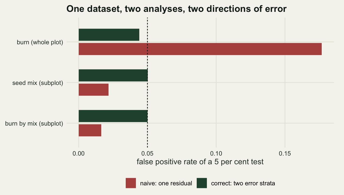
The correct analysis sits on the nominal level for all three terms: 0.044, 0.0503 and 0.05, each within about two Monte Carlo standard errors of 0.05. That is the baseline, and it says the hand-written decomposition is not quietly broken.
The single-residual analysis rejects the burn null 0.1767 of the time, 3.535 times the nominal rate. In the same fits it rejects the seed mix null 0.0217 of the time and the interaction null 0.0165 of the time, which is 0.435 and 0.33 times nominal. The subplot terms are not slightly conservative. They have lost most of their intended error budget, and some power with it.
There is no way to read this off a printed table. Both analyses give the same treatment sums of squares and the same estimated means. The only thing that differs is a denominator, and the denominator that is too small and the denominator that is too big are the same number.
The two errors also combine into a particular shape of wrong answer, and that is worth counting directly. The pattern an author would most like to find in a burning experiment is that the fire treatment matters and the seeding does not, because that is a clean story about disturbance. Ask how often a complete null delivers exactly that pattern under each analysis.
sig <- p_null < 0.05
tidy_story <- function(w, s) mean(sig[w, ] & !sig[s, ])
print(round(c(
  correct_fire_yes_seed_no = tidy_story("burn_correct", "mix_correct"),
  naive_fire_yes_seed_no = tidy_story("burn_naive", "mix_naive"),
  correct_any_false_positive =
    mean(sig["burn_correct", ] | sig["mix_correct", ] | sig["both_correct", ]),
  naive_any_false_positive =
    mean(sig["burn_naive", ] | sig["mix_naive", ] | sig["both_naive", ])), 4))
correct_fire_yes_seed_no naive_fire_yes_seed_no
0.0415 0.1710
correct_any_false_positive naive_any_false_positive
0.1325 0.2040 Under the correct analysis the tidy story arrives by chance in 0.0415 of null datasets, which is the whole-plot false positive rate of 0.044 thinned slightly by the runs where the seed mix also fires. Under the naive analysis it arrives in 0.171, a factor of 4.12 more often. The two errors do not cancel when you read the table as a whole; they compound into the one conclusion the design was least able to support.
Why the pooled denominator cannot be right for both
The direction of each error follows from the expected mean squares, and those are short enough to write down. With \(\sigma^2_p\) the whole-plot variance and \(\sigma^2_e\) the subplot variance, and \(S\) subplots per whole plot,
\[E[\text{MS}_{\text{whole-plot error}}] = \sigma^2_e + S\,\sigma^2_p, \qquad E[\text{MS}_{\text{subplot error}}] = \sigma^2_e .\]
The pooled residual of the naive model is a degrees-of-freedom weighted average of the two, so it lies strictly between them whenever \(\sigma^2_p > 0\). It is therefore too small as a denominator for the burn test and too large as a denominator for the two subplot tests, and it cannot be fixed by choosing a different \(\sigma^2_p\): there is no positive value that makes both ratios one.
ems_wpe <- sd_sub^2 + n_mix * sd_plot^2
ems_sub <- sd_sub^2
ems_pool <- (df_wpe * ems_wpe + df_sub * ems_sub) / (df_wpe + df_sub)

print(round(c(variance_ratio = sd_plot^2 / sd_sub^2,
              ems_whole_plot_error = ems_wpe, ems_subplot_error = ems_sub,
              ems_pooled = ems_pool), 4))
variance_ratio ems_whole_plot_error ems_subplot_error
0.500 2.500 1.000
ems_pooled
1.375 print(round(c(burn_denominator_ratio = ems_pool / ems_wpe,
mix_denominator_ratio = ems_pool / ems_sub), 4))burn_denominator_ratio mix_denominator_ratio
0.550 1.375 At the variance ratio used above, 0.5, the burn test is handed a denominator 0.55 of the size it should have and the seed mix test one 1.375 times the size it should have. Those two numbers are the whole mechanism.
Sweeping the ratio turns the algebra into two curves. Everything else is held fixed: same design, same block variance, same subplot variance, only the whole-plot variance moves.
set.seed(20260802)
n_swp <- 3000
ratios <- c(0, 0.05, 0.1, 0.2, 0.35, 0.5, 0.75, 1, 1.5, 2, 3, 5)

sweep_rate <- function(r) {
  rowMeans(replicate(n_swp, split_p(
    sim_split(n_block, n_burn, n_mix, sd_block, sqrt(r), sd_sub),
    n_block, n_burn, n_mix)) < 0.05)
}
sw <- data.frame(ratio = ratios,
                 t(vapply(ratios, sweep_rate, numeric(6))))
print(round(sw, 4))
ratio burn_correct mix_correct both_correct burn_naive mix_naive both_naive
1 0.00 0.0467 0.0517 0.0510 0.0487 0.0503 0.0517
2 0.05 0.0520 0.0507 0.0417 0.0650 0.0450 0.0373
3 0.10 0.0490 0.0527 0.0467 0.0847 0.0423 0.0370
4 0.20 0.0470 0.0460 0.0500 0.1057 0.0307 0.0327
5 0.35 0.0503 0.0530 0.0490 0.1487 0.0257 0.0220
6 0.50 0.0520 0.0513 0.0480 0.1857 0.0243 0.0147
7 0.75 0.0490 0.0423 0.0400 0.2250 0.0113 0.0087
8 1.00 0.0473 0.0483 0.0510 0.2637 0.0097 0.0077
9 1.50 0.0533 0.0460 0.0480 0.3073 0.0060 0.0023
10 2.00 0.0523 0.0507 0.0483 0.3463 0.0027 0.0033
11 3.00 0.0510 0.0487 0.0527 0.3787 0.0010 0.0013
12 5.00 0.0477 0.0477 0.0480 0.4067 0.0000 0.0000hit_ten <- approx(sw$burn_naive, sw$ratio, xout = 0.10)$y
print(round(c(replicates_per_point = n_swp,
naive_burn_at_zero_ratio = sw$burn_naive[1],
naive_mix_at_zero_ratio = sw$mix_naive[1],
ratio_where_naive_burn_doubles = hit_ten,
naive_burn_at_largest_ratio = sw$burn_naive[nrow(sw)],
naive_mix_at_largest_ratio = sw$mix_naive[nrow(sw)]), 4)) replicates_per_point naive_burn_at_zero_ratio
3000.0000 0.0487
naive_mix_at_zero_ratio ratio_where_naive_burn_doubles
0.0503 0.1730
naive_burn_at_largest_ratio naive_mix_at_largest_ratio
0.4067 0.0000 lab_swp <- c("burn, one residual", "seed mix, one residual",
"burn, two strata", "seed mix, two strata")
swp_long <- data.frame(
ratio = rep(sw$ratio, 4),
rate = c(sw$burn_naive, sw$mix_naive, sw$burn_correct, sw$mix_correct),
series = factor(rep(lab_swp, each = nrow(sw)), levels = lab_swp))
ggplot(swp_long, aes(ratio, rate, colour = series, shape = series)) +
geom_hline(yintercept = 0.05, linetype = "22", colour = te_pal$ink) +
geom_line(linewidth = 0.7) +
geom_point(size = 2.1) +
scale_colour_manual(values = c(te_pal$clay, te_pal$gold, te_pal$forest,
te_pal$sage), name = NULL) +
scale_shape_manual(values = c(17, 15, 16, 18), name = NULL) +
scale_y_continuous(limits = c(0, 0.45)) +
guides(colour = guide_legend(nrow = 2), shape = guide_legend(nrow = 2)) +
labs(x = "whole-plot variance / subplot variance",
y = "false positive rate",
title = "One pooled residual, two error rates") +
theme_te() +
theme(plot.margin = margin(8, 16, 4, 8))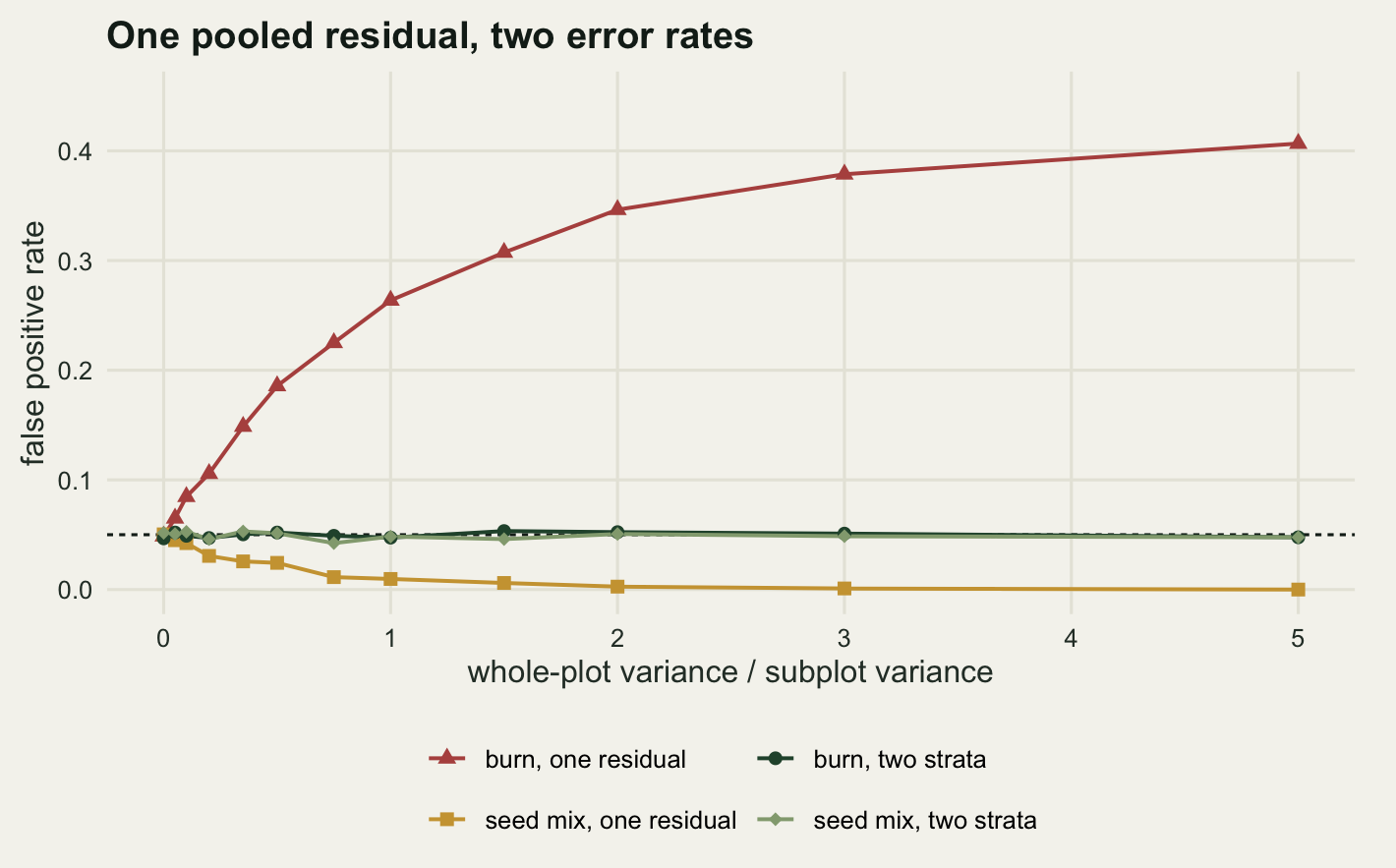
The question this sweep was built to answer is where the naive analysis is accidentally correct, and the answer is that there is no such place. At a ratio of zero the pooled residual estimates the same subplot variance as the two correct denominators, so the naive tests are valid by construction rather than by accident, and the measured naive rates are 0.0487 and 0.0503, both on target. Everywhere to the right of that the curves have already parted. They do not cross back, and there is no intermediate ratio at which the two errors cancel, because they are not two independent mistakes: they are one denominator being wrong in the only two ways a denominator can be wrong. I had expected a trade-off curve with an interior sweet spot. The expected mean squares rule it out before the simulation runs.
What the sweep does give is a scale for how quickly it matters. The naive burn test reaches twice its nominal rate at a variance ratio of about 0.173, meaning a whole-plot standard deviation of only 0.416 times the subplot standard deviation is enough to double the false positive rate. Field plots that differ by two fifths of a subplot standard deviation are not unusual; that is a small amount of heterogeneity to be doing this much damage. At the top of the range the naive burn rate is 0.4067 and the naive mix rate is 0, which is a test that has stopped being a test.
Where on that axis a real experiment sits is not something the analysis can tell you afterwards with any precision, because the whole-plot variance is estimated from 8 degrees of freedom. What sets it is the thing that made the whole plots large in the first place. Quarter hectare units cut across soil boundaries and drainage lines that a two-metre square never sees, and the coarser the unit the more of the site’s spatial structure ends up inside the whole-plot term rather than the subplot term. Larger whole plots move you to the right along this axis, which is the opposite of the intuition that bigger plots are more reliable.
Where the power goes
The two error strata are not only a hazard. They are also the reason the design is worth running, and that side of it is exactly measurable, because for a balanced design with normal errors each F statistic has an exact non-central F distribution. Writing \(Q\) for the sum of squared treatment effects of a term, the non-centrality parameters are
\[\lambda_{\text{burn}} = \frac{B S\, Q}{\sigma^2_e + S \sigma^2_p}, \qquad \lambda_{\text{mix}} = \frac{B W\, Q}{\sigma^2_e}, \qquad \lambda_{\text{burn} \times \text{mix}} = \frac{B\, Q}{\sigma^2_e}\]
with \(B\) blocks, \(W\) burn levels and \(S\) mix levels. Two things differ between the three: the denominator, and the multiplier in front. The subplot main effect gets the small error variance and averages each level over \(BW\) subplots. The interaction gets the small error variance too, and the whole-plot variance drops out of it completely, but each interaction cell mean is an average over only \(B\) subplots.
Give all three terms the same sum of squared effects so that only those structural differences are left, then compute exact power and check it by simulation.
delta <- 1.2
contr <- c(-1, 0, 1)
eff_burn <- delta * contr / 2
eff_mix <- delta * contr / 2
eff_both <- (delta / (2 * sqrt(2))) * outer(contr, contr)
q_eff <- c(burn = sum(eff_burn^2), mix = sum(eff_mix^2),
           both = sum(eff_both^2))
print(round(q_eff, 6))
burn mix both
0.72 0.72 0.72 pow_exact <- function(df1, df2, lam) {
1 - pf(qf(0.95, df1, df2), df1, df2, ncp = lam)
}
lambda_of <- function(r) {
qq <- q_eff[["burn"]]
c(burn = n_block * n_mix * qq / (sd_sub^2 + n_mix * r * sd_sub^2),
mix = n_block * n_burn * qq / sd_sub^2,
both = n_block * qq / sd_sub^2)
}
power_of <- function(r) {
lam <- lambda_of(r)
c(burn = pow_exact(n_burn - 1, df_wpe, lam[["burn"]]),
mix = pow_exact(n_mix - 1, df_sub, lam[["mix"]]),
both = pow_exact((n_burn - 1) * (n_mix - 1), df_sub, lam[["both"]]))
}
r_base <- sd_plot^2 / sd_sub^2
print(round(lambda_of(r_base), 4)) burn mix both
4.32 10.80 3.60 print(round(power_of(r_base), 4)) burn mix both
0.3190 0.7944 0.2426 set.seed(20260803)
n_pow <- 8000
sim_power <- function(r, which_eff) {
args <- list(rep(0, n_burn), rep(0, n_mix), matrix(0, n_mix, n_burn))
args[[which_eff]] <- switch(which_eff, eff_burn, eff_mix, eff_both)
mean(replicate(n_pow, split_p(
sim_split(n_block, n_burn, n_mix, sd_block, sqrt(r) * sd_sub, sd_sub,
args[[1]], args[[2]], args[[3]]),
n_block, n_burn, n_mix)[which_eff]) < 0.05)
}
pow_sim <- c(burn = sim_power(r_base, 1), mix = sim_power(r_base, 2),
both = sim_power(r_base, 3))
print(round(pow_sim, 4)) burn mix both
0.3191 0.7976 0.2484 print(round(c(replicates = n_pow,
max_abs_gap = max(abs(pow_sim - power_of(r_base))),
mc_se_at_half = sqrt(0.25 / n_pow)), 5)) replicates max_abs_gap mc_se_at_half
8.00e+03 5.82e-03 5.59e-03 At the base variance ratio the exact powers are 0.319 for the burn treatment, 0.7944 for the seed mix and 0.2426 for the interaction, against simulated values of 0.3191, 0.7976 and 0.2484. The largest gap is 0.00582, against a Monte Carlo standard error of about 0.00559, so the closed-form curves below can be trusted and drawn without simulation noise.
r_grid <- seq(0, 3, length.out = 121)
pw_grid <- t(vapply(r_grid, power_of, numeric(3)))
lab_pow <- c("burn (whole plot)", "seed mix (subplot)", "burn by mix (subplot)")
pw_long <- data.frame(
  ratio = rep(r_grid, 3),
  power = as.vector(pw_grid),
  term = factor(rep(lab_pow, each = length(r_grid)), levels = lab_pow))
chk <- data.frame(ratio = r_base, power = as.numeric(pow_sim),
                  term = factor(lab_pow, levels = lab_pow))

cross_r <- uniroot(function(r) power_of(r)[["both"]] - power_of(r)[["burn"]],
                   c(0.01, 10))$root

ggplot(pw_long, aes(ratio, power, colour = term)) +
  geom_line(linewidth = 0.8) +
  geom_point(data = chk, size = 3, shape = 21, fill = te_pal$paper) +
  scale_colour_manual(values = c(te_pal$clay, te_pal$green, te_pal$gold),
                      name = NULL) +
  scale_y_continuous(limits = c(0, 1)) +
  guides(colour = guide_legend(nrow = 2)) +
  labs(x = "whole-plot variance / subplot variance",
       y = "power of a 5 per cent test",
       title = "The same effect, three places to put it") +
  theme_te() +
  theme(plot.margin = margin(8, 16, 4, 8))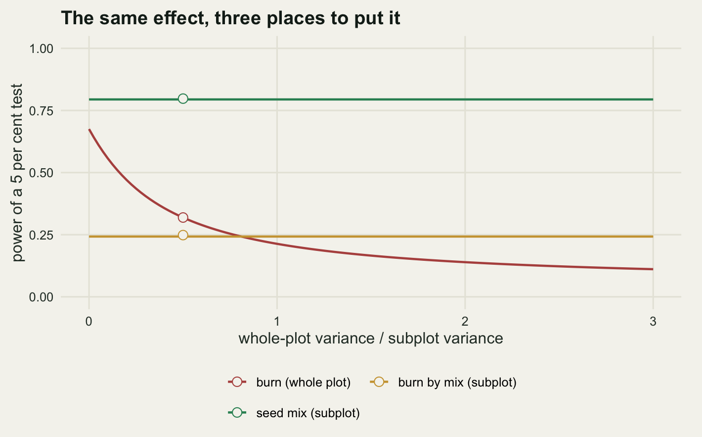
The seed mix line is flat at 0.7944 across the whole range, and so is the interaction line at 0.2426. Neither test can see the whole-plot variance, so making the plots more heterogeneous costs them nothing. The burn curve starts at 0.6751 when the whole plots are exchangeable and drops to 0.1112 by the right-hand edge. At the ratio used in the simulations the same effect is detected 0.7944 of the time at subplot level and 0.319 of the time at whole-plot level, a factor of 2.49.
Put a price on that gap and the advice gets sharper. The only way to raise the whole-plot power without moving the treatment is to add blocks, which means more quarter-hectare plots and more fire. Solve for how many.
pow_burn_blocks <- function(nb, r) {
  lam <- nb * n_mix * q_eff[["burn"]] / (sd_sub^2 * (1 + n_mix * r))
  pow_exact(n_burn - 1, (nb - 1) * (n_burn - 1), lam)
}
target <- power_of(r_base)[["mix"]]
blocks_try <- 3:40
pow_by_block <- vapply(blocks_try, pow_burn_blocks, numeric(1), r = r_base)
need <- blocks_try[which(pow_by_block >= target)[1]]

print(round(cbind(blocks = blocks_try, power = pow_by_block)[
  blocks_try %in% c(5, 10, 15, 20, need), ], 4))
blocks power
[1,] 5 0.3190
[2,] 10 0.6745
[3,] 13 0.8107
[4,] 15 0.8722
[5,] 20 0.9560print(round(c(target_power = target, blocks_needed = need,
whole_plots_needed = need * n_burn,
whole_plots_now = n_block * n_burn,
extra_whole_plots = (need - n_block) * n_burn,
subplots_needed = need * n_burn * n_mix), 3)) target_power blocks_needed whole_plots_needed whole_plots_now
0.794 13.000 39.000 15.000
extra_whole_plots subplots_needed
24.000 117.000 To give the burn treatment the power the seed mix already has, 0.7944, the experiment needs 13 blocks instead of 5. That is 39 whole plots against 15, so 24 more quarter-hectare units to burn, fence and monitor, for one factor. Nobody is funding that. The realistic move is the other one: decide before the season which question the experiment is for, and if the answer is the fire, accept that the seed mix is along for the ride rather than the reverse.
The design advice follows without hedging. The treatment you actually care about goes on the subplot if the logistics allow it at all. The one you are willing to describe loosely, or that you only need as a context for the other, goes on the whole plot. Splitting is not a compromise forced on you by fire crews; it is a way of buying precision for one factor at the price of precision for the other, and you get to choose which.
The interaction is where my expectation was wrong, and the figure shows it. The standard summary of a split-plot design says the subplot factor and the interaction are both tested with the better error term, which is true, and it is easy to slide from there to thinking both are more powerful than the whole-plot factor, which is not. At equal effect sum of squares the interaction sits at 0.2426, below the whole-plot factor’s 0.319. The non-centrality multipliers say why: the whole-plot main effect averages each level over 15 subplots against the interaction cell’s 5, which is a factor of 3 in its favour, and the interaction also spreads its signal over 4 degrees of freedom instead of 2. The better error term has to make up for both before it wins anything.
It does win eventually. The two curves cross at a variance ratio of 0.81, and beyond that the interaction is the more powerful of the two. That number is not universal; it depends on how many subplots the whole plot is cut into and how the effect is parametrised. What is general is the shape of the argument: the interaction is immune to whole-plot heterogeneity and pays for that immunity with replication, so whether it comes out ahead is an arithmetic question about your particular design, not a property of split-plot designs as such.
The mixed model gives the same answer, until the design is not balanced
The two-strata aov is a decomposition, not a model fit. A linear mixed model with random intercepts for block and for whole plot within block is the same statement written as a model, and on balanced data the two agree exactly.
nlme is used here rather than lme4 for one reason: it reports denominator degrees of freedom and an F test, so the comparison with the aov strata is direct. lme4 deliberately declines to report them, on the grounds that there is no generally correct answer once the design is unbalanced, which is the same point this section ends on from the other side.
library(nlme)

fit_lme <- lme(y ~ burn * mix, random = ~1 | block / burn, data = dd,
               method = "REML")
an_lme <- anova(fit_lme)
print(an_lme)
numDF denDF F-value p-value
(Intercept) 1 24 5.453013 0.0282
burn 2 8 0.299504 0.7491
mix 2 24 1.031109 0.3719
burn:mix 4 24 0.220176 0.9245f_aov <- c(grab(aov_tab[[2]], "burn", "F value"),
grab(aov_tab[[3]], "mix", "F value"),
grab(aov_tab[[3]], "burn:mix", "F value"))
f_lme <- an_lme[c("burn", "mix", "burn:mix"), "F-value"]
vc <- suppressWarnings(as.numeric(VarCorr(fit_lme)[c(2, 4, 5), "Variance"]))
print(round(c(block_var = vc[1], whole_plot_var = vc[2], resid_var = vc[3]), 4)) block_var whole_plot_var resid_var
0.2427 0.4275 1.1703 print(round(c(den_df_burn = an_lme["burn", "denDF"],
den_df_mix = an_lme["mix", "denDF"],
max_abs_f_gap = max(abs(f_aov - f_lme))), 8)) den_df_burn den_df_mix max_abs_f_gap
8.0e+00 2.4e+01 1.0e-08 The denominator degrees of freedom the mixed model chooses are 8 for the burn effect and 24 for the seed mix, which are the two residual lines of the aov output. The F statistics match to 1.39e-08. The variance components are the same information in a different shape: 0.4275 between whole plots within a block against 1.1703 between subplots, whose ratio is 0.3653 and whose generating value was 0.5.
That exactness has one condition, and it is worth finding out how often the condition fails. Then remove the balance and watch the two approaches separate. The thinning below drops one subplot from each of five whole plots, a deliberately mild unbalancing: forty of forty-five subplots survive and every whole plot keeps at least two.
p_terms_aov <- function(fit, term) {
  s <- summary(fit)
  out <- numeric(0)
  for (nm in names(s)) {
    tb <- s[[nm]][[1]]
    rn <- trimws(rownames(tb))
    if (term %in% rn) out <- c(out, tb[rn == term, "Pr(>F)"])
  }
  out[!is.na(out)]
}
thin_design <- function(d, k) {
  hit <- sample(levels(d$plot), k)
  d[-vapply(hit, function(p) sample(which(d$plot == p), 1), integer(1)), ]
}

set.seed(20260806)
n_rep <- 60
n_thin <- 5
cmp <- do.call(rbind, lapply(seq_len(n_rep), function(i) {
  d <- make_design(n_block, n_burn, n_mix)
  d$y <- sim_split(n_block, n_burn, n_mix, sd_block, sd_plot, sd_sub,
                   eff_w = 0.45 * contr, eff_s = 0.45 * contr)
  du <- thin_design(d, n_thin)
  pb <- p_terms_aov(aov(y ~ burn * mix + Error(block / burn), data = d), "mix")
  pu <- p_terms_aov(aov(y ~ burn * mix + Error(block / burn), data = du), "mix")
  mb <- lme(y ~ burn * mix, random = ~1 | block / burn, data = d,
            method = "REML")
  mu <- lme(y ~ burn * mix, random = ~1 | block / burn, data = du,
            method = "REML")
  vb <- suppressWarnings(as.numeric(VarCorr(mb)[c(2, 4, 5), "Variance"]))
  data.frame(rep = i, bal_aov = pb[length(pb)],
             bal_lme = anova(mb)["mix", "p-value"],
             unb_aov = pu[length(pu)], unb_lme = anova(mu)["mix", "p-value"],
             unb_strata = length(pu), wp_var = vb[2])
}))
cmp$interior <- cmp$wp_var > 1e-6

print(round(c(datasets = n_rep, subplots_dropped = n_thin,
              interior_fits = sum(cmp$interior),
              boundary_fits = sum(!cmp$interior)), 3))
datasets subplots_dropped interior_fits boundary_fits
60 5 54 6 print(signif(c(
bal_max_gap_interior = max(abs(cmp$bal_aov - cmp$bal_lme)[cmp$interior]),
bal_max_gap_boundary = max(abs(cmp$bal_aov - cmp$bal_lme)[!cmp$interior]),
unbal_max_gap = max(abs(cmp$unb_aov - cmp$unb_lme)),
unbal_median_gap = median(abs(cmp$unb_aov - cmp$unb_lme))), 4))bal_max_gap_interior bal_max_gap_boundary unbal_max_gap
1.399e-06 3.749e-02 1.469e-01
unbal_median_gap
1.110e-02 print(round(c(unbal_terms_in_two_or_more_strata = mean(cmp$unb_strata > 1),
unbal_verdict_flips_at_05 =
mean((cmp$unb_aov < 0.05) != (cmp$unb_lme < 0.05))), 4))unbal_terms_in_two_or_more_strata unbal_verdict_flips_at_05
1.0000 0.0667 kind_lv <- c("balanced, interior variance estimate",
"balanced, variance estimate at zero", "five subplots dropped")
mix_pts <- rbind(
data.frame(aovp = cmp$unb_aov, lmep = cmp$unb_lme, kind = kind_lv[3]),
data.frame(aovp = cmp$bal_aov[cmp$interior], lmep = cmp$bal_lme[cmp$interior],
kind = kind_lv[1]),
data.frame(aovp = cmp$bal_aov[!cmp$interior],
lmep = cmp$bal_lme[!cmp$interior], kind = kind_lv[2]))
mix_pts$kind <- factor(mix_pts$kind, levels = kind_lv)
ggplot(mix_pts, aes(lmep, aovp, colour = kind, shape = kind)) +
geom_abline(slope = 1, intercept = 0, linetype = "22", colour = te_pal$ink) +
geom_hline(yintercept = 0.05, colour = te_pal$sage, linewidth = 0.7) +
geom_vline(xintercept = 0.05, colour = te_pal$sage, linewidth = 0.7) +
geom_point(size = 2.4, alpha = 0.9) +
scale_x_log10() +
scale_y_log10() +
scale_colour_manual(values = c(te_pal$forest, te_pal$gold, te_pal$clay),
name = NULL) +
scale_shape_manual(values = c(16, 15, 17), name = NULL) +
guides(colour = guide_legend(nrow = 2), shape = guide_legend(nrow = 2)) +
labs(x = "p-value from the mixed model",
y = "p-value from the two-strata aov",
title = "Where the two routes stop agreeing") +
theme_te() +
theme(plot.margin = margin(8, 16, 4, 8))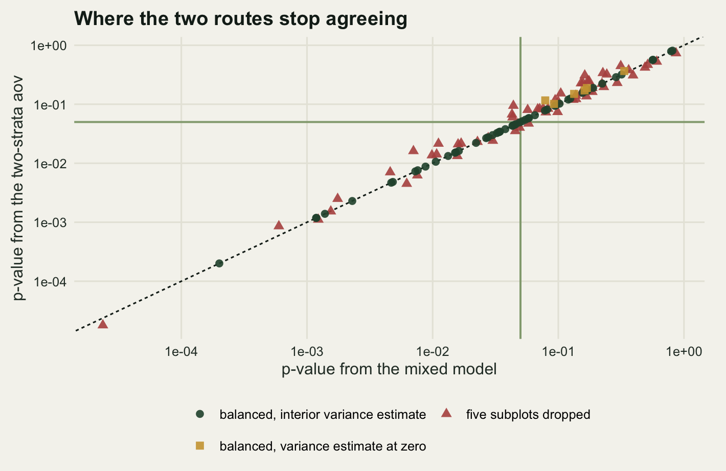
Of the 60 balanced datasets, 54 had the whole-plot variance estimated strictly inside the parameter space, and on those the two p-values agree to 1.4e-06, which is optimiser tolerance. The other 6 are the condition failing. When the whole-plot mean square comes out below the subplot mean square, the method-of-moments estimate of the whole-plot variance is negative, and the two approaches part company over what to do about it. The mixed model sets it to zero and pools the two error terms; aov keeps the strata apart, so the seed mix test still divides by the subplot mean square. The largest disagreement among those fits is 0.03749 on the p-value scale.
Unbalancing the design breaks the agreement structurally rather than occasionally. In every one of the 60 thinned datasets the seed mix term appeared in more than one error stratum of the aov output, because it is no longer orthogonal to blocks and whole plots. There is no single F for it any more, only a piece of it in each stratum, and picking the one from the Within table is a convention rather than a result. That convention disagrees with the mixed model by a median of 0.0111 on the p-value scale and by up to 0.1469, and it moves the verdict across the five per cent line in 7 per cent of the datasets after dropping 5 subplots out of 45.
Five missing subplots is nothing. A grazing exclosure blows over, a subplot floods, a sample is lost in the lab, and the balance a split-plot aov needs is gone. Use aov with an Error term to see the two strata written out and to check that you have understood the design; fit the mixed model to get the answer.
What to take away
The measurement is that one residual line produces two errors at once. In 4000 null datasets the single-residual analysis rejected the whole-plot null 0.1767 of the time and the subplot null 0.0217 of the time, against a nominal 0.05 and a correct analysis that sat at 0.044 and 0.0503. The whole-plot treatment gets credit it has not earned and the subplot treatment is held to a standard nobody set.
The expected mean squares say this cannot be tuned away. The pooled residual lies between \(\sigma^2_e\) and \(\sigma^2_e + S\sigma^2_p\) for any positive whole-plot variance, and the sweep found no ratio at which both tests come right: at a ratio of 0 they were both correct because the pooled residual then estimates the same subplot variance as the two correct denominators, and by a ratio of 0.173 the whole-plot false positive rate had already doubled.
On the design side, the ordering of the exact powers at the base configuration was 0.7944 for the subplot factor, 0.319 for the whole-plot factor and 0.2426 for the interaction. The first comparison is the design advice: put the question you care about at the subplot level. The second was the surprise. The interaction has the better error term and still less power than the whole-plot factor here, because an interaction cell is an average over 5 subplots rather than 15, and it only overtakes the whole-plot factor once the variance ratio passes 0.81.
The honest limit is that everything above is a balanced-design result, and balance is the first thing a field season destroys. The exact non-central F powers, the clean two-stratum decomposition and the exact agreement with the mixed model all assumed every whole plot had 3 subplots. Drop 5 of 45 and the seed mix term scattered across more than one stratum in every one of 60 datasets, with the conventional choice of stratum flipping the five per cent verdict in 7 per cent of them. The power calculation you do before the season is a balanced-design calculation; the analysis you do after it will not be, and the gap between those two is not something this post has measured.
References
Yates F 1935 Journal of the Royal Statistical Society Series B 2(2):181-223 (10.2307/2983638)
Hurlbert SH 1984 Ecological Monographs 54(2):187-211 (10.2307/1942661)
Millar RB, Anderson MJ 2004 Fisheries Research 70(2-3):397-407 (10.1016/j.fishres.2004.08.016)
Schielzeth H, Nakagawa S 2013 Methods in Ecology and Evolution 4(1):14-24 (10.1111/j.2041-210X.2012.00251.x)
Bolker BM, Brooks ME, Clark CJ, Geange SW, Poulsen JR, Stevens MHH, White JSS 2009 Trends in Ecology and Evolution 24(3):127-135 (10.1016/j.tree.2008.10.008)
Kenward MG, Roger JH 2009 Computational Statistics and Data Analysis 53(7):2583-2595 (10.1016/j.csda.2008.12.013)
Quinn GP, Keough MJ 2002 Experimental Design and Data Analysis for Biologists (ISBN 978-0-521-00976-8)
Pinheiro JC, Bates DM 2000 Mixed-Effects Models in S and S-PLUS (ISBN 978-0-387-98957-0)