library(ggplot2)
library(patchwork)

te_paper  <- "#f5f4ee"
te_ink    <- "#16241d"
te_body   <- "#2c3a31"
te_forest <- "#275139"
te_rust   <- "#b5534e"
te_gold   <- "#c9b458"
te_line   <- "#dad9ca"

theme_datasheet <- function() {
  theme_minimal(base_size = 12) +
    theme(plot.background  = element_rect(fill = te_paper, colour = NA),
          panel.background = element_rect(fill = te_paper, colour = NA),
          panel.grid.major = element_line(colour = te_line, linewidth = 0.3),
          panel.grid.minor = element_blank(),
          text             = element_text(colour = te_body),
          plot.title       = element_text(colour = te_ink, face = "bold"),
          plot.subtitle    = element_text(colour = te_body),
          axis.text        = element_text(colour = te_body))
}Random effects with too few levels
R
mixed models
variance components
simulation
ecology tutorial
With five streams the variance component is most often exactly zero. Measuring in R why dropping that singular random term barely harms a group-level test.
Five headwater streams along a catchment logging gradient, four riffle samples in each, twenty samples of shredder biomass in total. The design is modest but it is the design most people actually get: streams are expensive, riffles are cheap, and the permit covers one field season. The question is whether shredder biomass falls with the proportion of the catchment logged, and the covariate is a property of the stream, not of the riffle.
Fit a random intercept for stream and the variance component often comes back as zero. The fit is reported as singular, the summary looks wrong, and the next step is almost always the same: remove the random term, refit with plain least squares on all twenty samples, report that p value.
That zero is not a surprise, and this site has already measured it. The post on the parametric bootstrap simulated null datasets for a non-negative dispersion parameter and found slightly more than half of the simulated statistics sitting exactly at zero. The asymptotic answer there is exactly one half, because a parameter pinned to a boundary under the null contributes a point mass of that size; only the small excess above a half is a small sample effect. The post on nested and crossed random effects lists the same boundary among its honest limits, warning that in a generalised linear mixed model a variance component of zero is a boundary and the fitting machinery has its own reasons to end up there. So the boundary is old news here. What this post measures is what happens after the boundary: the reflex of deleting the random term from a singular fit, and what that decision rule does to the test and the interval for the stream level covariate.
The estimator is not new here either. The post on variance components in monitoring data builds a moment estimator of the same family from mean squares in base R, with no package, but it is a two way split of site, year, site by year and residual variance rather than the one way split used here. It writes the components as plain differences of mean squares, without the truncation at zero, and it never asks how often the difference comes out negative. That frequency is the quantity this post is built around.
Five streams and four riffles is a real design
The generating model is the balanced one way random effects model with a group level covariate: each stream gets an intercept drawn from a normal distribution, each riffle sample adds independent noise, and the logging covariate is constant inside a stream.
n_strm  <- 5                        # streams
n_per   <- 4                        # riffle samples per stream
icc_set <- 0.10                     # intraclass correlation of the truth
v_a     <- icc_set                  # among stream variance, total variance one
v_e     <- 1 - v_a                  # within stream variance
mu0     <- 1.2                      # mean log biomass
slope_set <- -0.12                  # per ten percentage points logged
alpha_lev <- 0.05; ci_pct <- 100 * (1 - alpha_lev)

# catchment logged, five to eighty five per cent, in tens of points, centred
gradient_c <- function(J) {
  pct <- seq(5, 85, length.out = J) / 10
  pct - mean(pct)
}

make_streams <- function(J, n_per, slope, va, ve) {
  xg <- gradient_c(J)
  dat <- data.frame(stream = factor(rep(seq_len(J), each = n_per)),
                    logged = rep(xg, each = n_per))
  dat$y <- mu0 + slope * dat$logged +
           rep(rnorm(J, 0, sqrt(va)), each = n_per) + rnorm(J * n_per, 0, sqrt(ve))
  dat
}
In a balanced design the moment estimator of the among stream variance is closed form, so no fitting algorithm is involved and nothing can fail to converge. Two least squares fits give it. One regresses the response on stream identity and returns the within stream mean square. The other regresses the five stream means on the logging covariate; its residual mean square has expectation equal to the among stream variance plus the within stream variance divided by the number of samples per stream. Subtracting gives the estimate, and the truncation at zero is applied by hand.
vc_moment <- function(dat, n_per) {
  m_within <- lm(y ~ stream, data = dat)
  ms_e <- deviance(m_within) / df.residual(m_within)
  agg  <- aggregate(y ~ stream + logged, data = dat, FUN = mean)
  m_means <- lm(y ~ logged, data = agg)
  ms_m <- deviance(m_means) / df.residual(m_means)
  list(ms_e = ms_e, ms_m = ms_m,
       raw    = ms_m - ms_e / n_per,          # unbiased, can be negative
       sig_a2 = max(0, ms_m - ms_e / n_per),  # what software reports
       m_means = m_means, m_pool = lm(y ~ logged, data = dat))
}
set.seed(3116)
draws <- lapply(seq_len(6), function(i) make_streams(n_strm, n_per, slope_set, v_a, v_e))
vc_draws <- vapply(draws, function(d) vc_moment(d, n_per)$sig_a2, 0)
n_zero_draws <- sum(vc_draws == 0)
round(vc_draws, 3)
[1] 0.000 0.239 0.000 0.000 0.481 0.055Six datasets from one generating process, identical in every respect except the random draw, and 3 of the 6 return a stream variance of exactly zero against a true value of 0.10. Nothing has gone wrong in those datasets. The difference of mean squares came out negative and was truncated.
The two analyses that follow from one singular dataset are worth putting side by side. The regression on the five stream means keeps the stream level structure; the pooled regression on all twenty samples throws it away.
i_zero <- which(vc_draws == 0)[1]
ex <- vc_moment(draws[[i_zero]], n_per)
keep_row <- summary(ex$m_means)$coefficients["logged", ]
pool_row <- summary(ex$m_pool)$coefficients["logged", ]
ex_slope <- unname(keep_row[1]); ex_se_keep <- unname(keep_row[2])
ex_se_pool <- unname(pool_row[2]); df_pool <- df.residual(ex$m_pool)
ex_p_keep <- unname(keep_row[4]); ex_p_pool <- unname(pool_row[4])
df_keep <- df.residual(ex$m_means)
Both fits return the same slope, -0.0332 log units per ten percentage points logged, because the design is balanced and the covariate is constant within a stream. What differs is the uncertainty. The stream means regression gives a standard error of 0.0577 on 3 degrees of freedom and a p value of 0.605; the pooled regression gives 0.0699 on 18 degrees of freedom and a p value of 0.641. In this dataset the pooled standard error is the larger of the two, which is already a hint that the reflex does not behave the way it is usually described.
The estimate on the boundary is the estimator working
Measuring the boundary rate means repeating this thousands of times, and repeating two least squares fits is slow. In a balanced Gaussian design the fits depend on the data only through the stream means and the within stream sum of squares, and both have known distributions: the stream means are normal with variance equal to the among stream variance plus the within stream variance over the number of samples, and the within stream sum of squares is the within stream variance times a chi squared variate. Drawing those directly is exact rather than approximate, but that is a claim to check, not to assert.
analyse_suff <- function(ybar, ss_e, J, n_per, alpha = alpha_lev) {
  xg  <- gradient_c(J); sxx <- sum(xg^2)
  ctr <- ybar - rep(colMeans(ybar), each = J)
  slope_hat <- as.vector(crossprod(xg, ctr)) / sxx
  rss_m <- colSums((ctr - outer(xg, slope_hat))^2)
  dfp   <- J * n_per - 2
  ms_m  <- rss_m / (J - 2)
  ms_e  <- ss_e / (J * (n_per - 1))
  list(slope_hat = slope_hat, ms_m = ms_m, ms_e = ms_e,
       raw = ms_m - ms_e / n_per,
       se_keep = sqrt(ms_m / sxx),
       se_pool = sqrt((ss_e + n_per * rss_m) / dfp / (n_per * sxx)),
       crit_keep = qt(1 - alpha / 2, J - 2), crit_pool = qt(1 - alpha / 2, dfp))
}
i_pos <- which(vc_draws > 0)[1]
ybar_obs <- as.vector(tapply(draws[[i_pos]]$y, draws[[i_pos]]$stream, mean))
ss_e_obs <- sum((draws[[i_pos]]$y - ybar_obs[as.integer(draws[[i_pos]]$stream)])^2)
chk <- analyse_suff(matrix(ybar_obs, nrow = n_strm), ss_e_obs, n_strm, n_per)
ref <- vc_moment(draws[[i_pos]], n_per)
id_gap <- max(abs(c(chk$slope_hat - unname(coef(ref$m_means)["logged"]),
                    chk$se_keep - summary(ref$m_means)$coefficients["logged", 2],
                    chk$se_pool - summary(ref$m_pool)$coefficients["logged", 2],
                    chk$raw - ref$raw)))
On a dataset that did not land on the boundary the two routes agree to 5.6e-17, which is rounding error: the shortcut reproduces the slope, both standard errors and the variance estimate exactly.
The boundary probability also has a closed form. The estimate is negative when the mean square of the stream means falls below the within stream mean square divided by the number of samples per stream, and the ratio of those two mean squares is a scaled F variate, so the probability is one call to pf. That is a third, independent check.
sim_fast <- function(n_rep, J, n_per, slope, va, ve) {
  xg <- gradient_c(J)
  ybar <- matrix(rnorm(n_rep * J, 0, sqrt(va + ve / n_per)), nrow = J) + slope * xg
  analyse_suff(ybar, ve * rchisq(n_rep, J * (n_per - 1)), J, n_per)
}
p_zero_exact <- function(J, n_per, va, ve) pf((ve / n_per) / (va + ve / n_per), J - 2, J * (n_per - 1))
n_rep <- 20000    # fixed before any rate was inspected
n_chk <- 4000     # cross-check, full least squares on every dataset
set.seed(8140)
full_raw <- vapply(seq_len(n_chk), function(i)
  vc_moment(make_streams(n_strm, n_per, 0, v_a, v_e), n_per)$raw, 0)
set.seed(8141)
rate_chk   <- mean(sim_fast(n_chk, n_strm, n_per, 0, v_a, v_e)$raw <= 0)
rate_full <- mean(full_raw <= 0)
rate_exact <- p_zero_exact(n_strm, n_per, v_a, v_e)
chk_gap <- max(abs(c(rate_full, rate_chk) - rate_exact))
mcse_chk <- sqrt(0.25 / n_chk); mcse_rep <- sqrt(0.25 / n_rep)
The full least squares simulation puts the boundary rate at 0.429, the shortcut at 0.423 and the closed form at 0.429. The largest gap is 0.006, against a Monte Carlo standard error of at most 0.008 for a run of 4000. Everything below uses the shortcut with 20000 replicates, a count fixed before any rate was looked at, which holds the Monte Carlo standard error below 0.0035 for any rate.
procs <- function(a, slope_true = 0) {
  zero <- a$raw <= 0
  rej_keep <- abs(a$slope_hat / a$se_keep) > a$crit_keep
  rej_pool <- abs(a$slope_hat / a$se_pool) > a$crit_pool
  cov_k <- abs(a$slope_hat - slope_true) <= a$crit_keep * a$se_keep
  cov_p <- abs(a$slope_hat - slope_true) <= a$crit_pool * a$se_pool
  list(zero = zero, keep = rej_keep, pool = rej_pool, cov_keep = cov_k,
       adapt = ifelse(zero, rej_pool, rej_keep), cov_pool = cov_p,
       cov_adapt = ifelse(zero, cov_p, cov_k),
       w_keep = 2 * a$crit_keep * a$se_keep, w_pool = 2 * a$crit_pool * a$se_pool,
       w_adapt = ifelse(zero, 2 * a$crit_pool * a$se_pool, 2 * a$crit_keep * a$se_keep))
}
set.seed(2731)
main <- sim_fast(n_rep, n_strm, n_per, 0, v_a, v_e)
pm <- procs(main)
rate_main <- mean(pm$zero); mean_raw <- mean(main$raw)
mean_trunc <- mean(pmax(0, main$raw)); bias_trunc <- mean_trunc - v_a
Across 20000 datasets with no slope at all, 43.6 per cent of the estimates sit exactly on zero. Zero is a point mass and every other value has probability zero, so zero is the single most likely answer this design can give, by a wide margin. The untruncated difference of mean squares averages 0.097 against a true value of 0.10, so the estimator is unbiased before the truncation. Applying max(0, .) raises the average to 0.152, a bias of +0.052. Truncation is what makes the reported estimate biased upward, and it is also what stops it being a negative variance.
bd <- data.frame(raw = main$raw)
bd$side <- ifelse(bd$raw <= 0, "truncated to zero", "reported as positive")
ggplot(bd, aes(raw, fill = side)) +
  geom_histogram(bins = 70, colour = te_paper, linewidth = 0.15) +
  geom_vline(xintercept = v_a, colour = te_ink, linetype = "dashed", linewidth = 0.8) +
  scale_fill_manual(values = c(te_forest, te_rust), name = NULL) +
  labs(x = "estimated among stream variance, before truncation", y = "datasets",
       title = "Where the moment estimate lands with five streams",
       subtitle = "dashed line: the true among stream variance") +
  theme_datasheet() + theme(legend.position = "bottom")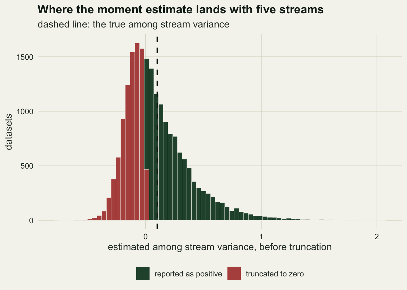
More streams, not more riffles, moves what matters
The boundary rate falls as streams are added, and it also falls as riffle samples are added, because both raise the expected ratio of the two mean squares. That is the honest version, and it is worth saying plainly, because the usual advice to add levels rather than replicates is not true of the boundary rate on its own.
Where the advice is true is in the quantity the study exists for. The standard error of the stream level slope is the square root of the among stream variance plus the within stream variance over the number of samples, divided by the spread of the covariate across streams. Only the second term shrinks with riffle samples, so there is a floor: no amount of within stream replication pushes the standard error below the value set by the among stream variance alone. Adding streams moves the floor itself and adds degrees of freedom to the test at the same time. Gelman and Hill 2007 make the same point in their chapter on sample size for multilevel models, where the number of groups, not the number of observations, drives what a group level coefficient can say.
j_seq <- c(4, 5, 6, 8, 10, 14, 20, 30)
n_lab <- c(4, 16)
rate_lev <- sprintf("%d per stream", n_lab)
rate_tab <- do.call(rbind, lapply(n_lab, function(nn)
  data.frame(J = j_seq, n_per = nn,
             rate = vapply(j_seq, function(J) p_zero_exact(J, nn, v_a, v_e), 0),
             label = factor(sprintf("%d per stream", nn), levels = rate_lev))))
set.seed(5504)
rate_sim <- vapply(j_seq, function(J) mean(sim_fast(n_rep, J, n_per, 0, v_a, v_e)$raw <= 0), 0)
sim_tab <- data.frame(J = j_seq, rate = rate_sim,
                      label = factor(rate_lev[1], levels = rate_lev))
sim_exact_gap <- max(abs(rate_sim - rate_tab$rate[rate_tab$n_per == n_per]))
r_at <- function(J) p_zero_exact(J, n_per, v_a, v_e)
se_slope <- function(J, nn) sqrt((v_a + v_e / nn) / sum(gradient_c(J)^2))
n_seq <- 2:40
j_lab <- c(5, 25); se_lev <- sprintf("%d streams", j_lab)
se_tab <- do.call(rbind, lapply(j_lab, function(J)
  data.frame(n_per = n_seq, J = J, se = vapply(n_seq, function(nn) se_slope(J, nn), 0),
             label = factor(sprintf("%d streams", J), levels = se_lev))))
floor_tab <- data.frame(J = j_lab, label = factor(se_lev, levels = se_lev),
      floor_se = vapply(j_lab, function(J) sqrt(v_a / sum(gradient_c(J)^2)), 0))
se_now <- se_slope(5, n_per); se_j25 <- se_slope(25, n_per)
se_gain5 <- se_now / floor_tab$floor_se[1]
With four samples per stream the closed form boundary rate is 42.9 per cent at five streams, 30.5 per cent at ten, 19.5 per cent at twenty and 13.5 per cent at thirty. Simulation agrees with the closed form to 0.003 across that range.
The floor is the sharper number. At five streams the slope standard error is 0.0901 with four samples each, and unlimited sampling within those same five streams would take it only to 0.0500. All the within stream replication in the world is worth a factor of 1.80. Twenty five streams with four samples each gives 0.0474, already below the five stream floor, and its own floor is 0.0263.
p_rate <- ggplot(rate_tab, aes(J, rate, colour = label)) +
  geom_line(linewidth = 0.9) +
  geom_point(data = sim_tab, shape = 21, size = 2.2, fill = te_paper,
             stroke = 0.8, show.legend = FALSE) +
  scale_colour_manual(values = c(te_forest, te_gold), name = NULL) +
  scale_y_continuous(limits = c(0, 0.5)) +
  labs(x = "streams", y = "probability of a zero estimate", title = "Boundary rate",
       subtitle = "lines: closed form, circles: simulation") +
  theme_datasheet() + theme(legend.position = "bottom")

p_se <- ggplot(se_tab, aes(n_per, se, colour = label)) +
  geom_line(linewidth = 0.9) +
  geom_hline(data = floor_tab, aes(yintercept = floor_se, colour = label),
             linetype = "dashed", linewidth = 0.6) +
  scale_colour_manual(values = c(te_forest, te_gold), name = NULL) +
  scale_y_continuous(limits = c(0, NA)) +
  labs(x = "riffle samples per stream", y = "standard error of the slope",
       title = "Precision of the slope",
       subtitle = "dashed lines: the variance floor") +
  theme_datasheet() + theme(legend.position = "bottom")

p_rate + p_se + plot_annotation(theme = theme_datasheet())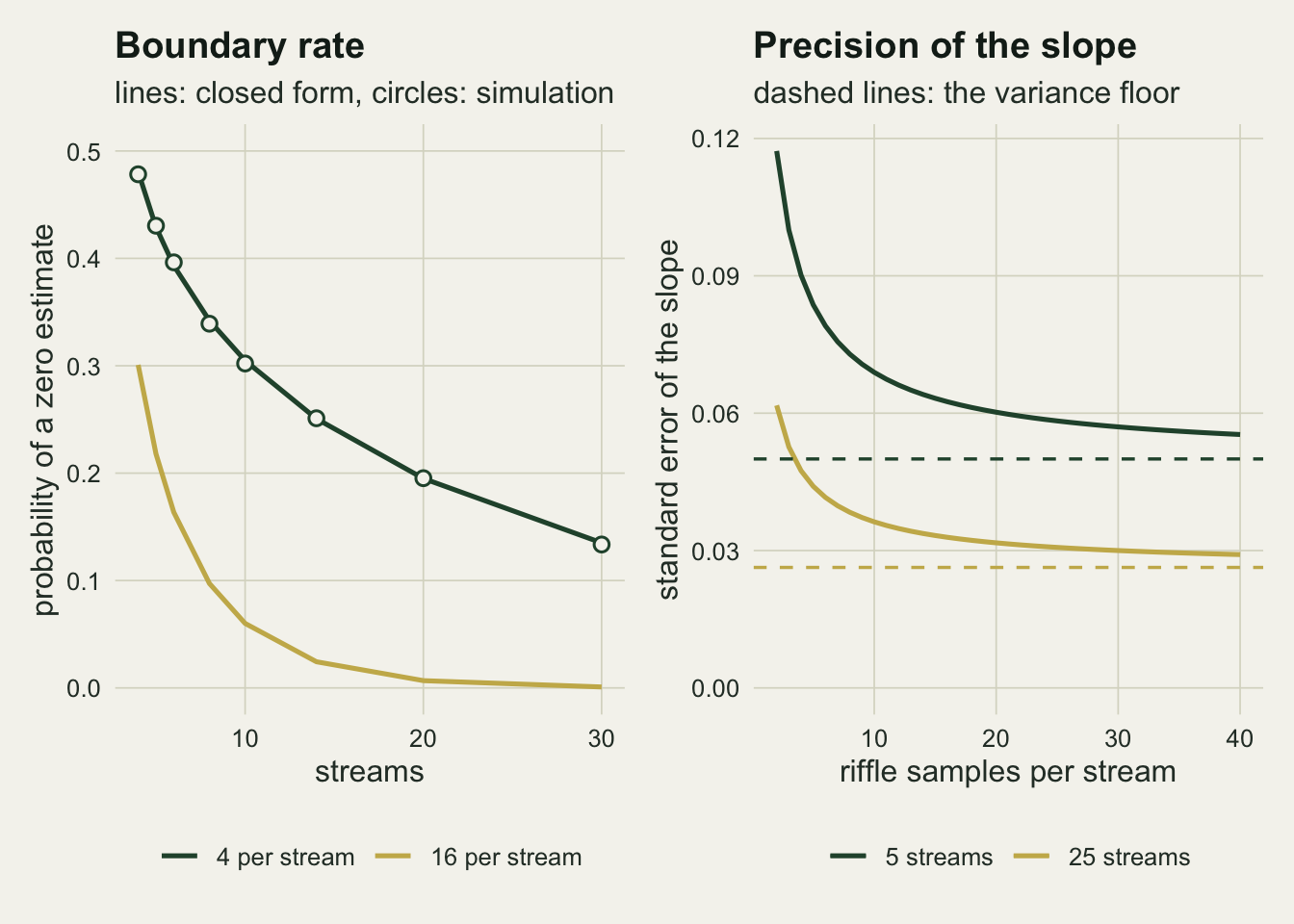
Dropping the term does less damage than the folklore says
Three procedures, applied to the same simulated datasets, all testing the stream level slope at a nominal five per cent. The first keeps the stream structure whatever the variance estimate does, which here is the regression on the stream means with its own degrees of freedom. The second is the reflex: if the variance estimate is zero, delete the random term and test on the residual degrees of freedom of all twenty samples, otherwise keep the structure. The third never fits a stream term at all.
proc_lev <- c("keep the term", "drop if singular", "always pool")
set.seed(6613)
ti <- do.call(rbind, lapply(j_seq, function(J) {
  pp <- procs(sim_fast(n_rep, J, n_per, 0, v_a, v_e))
  data.frame(J = J, procedure = proc_lev,
             rate = c(mean(pp$keep), mean(pp$adapt), mean(pp$pool)))
}))
ti$procedure <- factor(ti$procedure, levels = proc_lev)
ti$mcse <- sqrt(ti$rate * (1 - ti$rate) / n_rep)
at_j <- function(J, k) ti$rate[ti$J == J & ti$procedure == proc_lev[k]]
mcse_main <- sqrt(alpha_lev * (1 - alpha_lev) / n_rep)
rate_max <- function(k) max(ti$rate[ti$procedure == proc_lev[k]])
pool_max <- rate_max(3); adapt_max <- rate_max(2)
sing <- pm$zero; crit_ratio <- main$crit_keep / main$crit_pool
se_ratio_med <- median(main$se_pool[sing] / main$se_keep[sing])
thr_sing <- (main$crit_pool * main$se_pool[sing]) / (main$crit_keep * main$se_keep[sing])
thr_ratio_med <- median(thr_sing); thr_up <- mean(thr_sing[pm$keep[sing]] > 1)
At five streams the procedure that keeps the stream term rejects a true null 5.2 per cent of the time, which is what an exact test should do. The reflex rejects 4.3 per cent, and the fully pooled test 8.8 per cent. The Monte Carlo standard error near five per cent is 0.2 percentage points, so the gap between the first two is real but small, and it runs the wrong way for the folklore: the rule that deletes the random term is slightly conservative, not liberal.
At thirty streams the three rates are 5.1, 4.9 and 8.7 per cent. Adding streams repairs the reflex, because it triggers much less often, and it does nothing for the pooled test, whose worst rate across that range of stream counts is 8.8 per cent against 4.9 per cent for the reflex.
Why the reflex survives is worth stating, because it is not a general licence. The singular fit happens exactly when the stream means lie close to the fitted line, which is exactly when the mean square driving the correct standard error is small. Substituting the pooled standard error at that moment puts back a denominator built mostly from within stream noise. Across the singular datasets it multiplies the standard error by a median factor of 1.34, while the critical value falls by a factor of 1.51 as the degrees of freedom go from 3 to 18. The two moves are close in size, but they do not cancel: the median rejection threshold ends up 0.88 times the one it replaced, and yet among the singular datasets in which the correct test does reject, the pooled threshold is the higher of the two 74 per cent of the time. That asymmetry is why the rule lands on the conservative side. Bates and colleagues 2015 describe the singular fit as a report about the data rather than a failure of the algorithm, and this is what that looks like downstream.
ggplot(ti, aes(J, rate, colour = procedure)) +
  geom_hline(yintercept = alpha_lev, colour = te_body, linetype = "dashed",
             linewidth = 0.5) +
  geom_errorbar(aes(ymin = rate - 2 * mcse, ymax = rate + 2 * mcse),
                width = 0.6, linewidth = 0.4) +
  geom_line(linewidth = 0.9) + geom_point(size = 2.2) +
  scale_colour_manual(values = c(te_forest, te_gold, te_rust), name = NULL) +
  scale_y_continuous(limits = c(0, NA)) +
  labs(x = "streams", y = "rejection rate under the null",
       title = "Deleting the term barely moves the test",
       subtitle = "dashed line: the nominal five per cent") +
  theme_datasheet() + theme(legend.position = "bottom")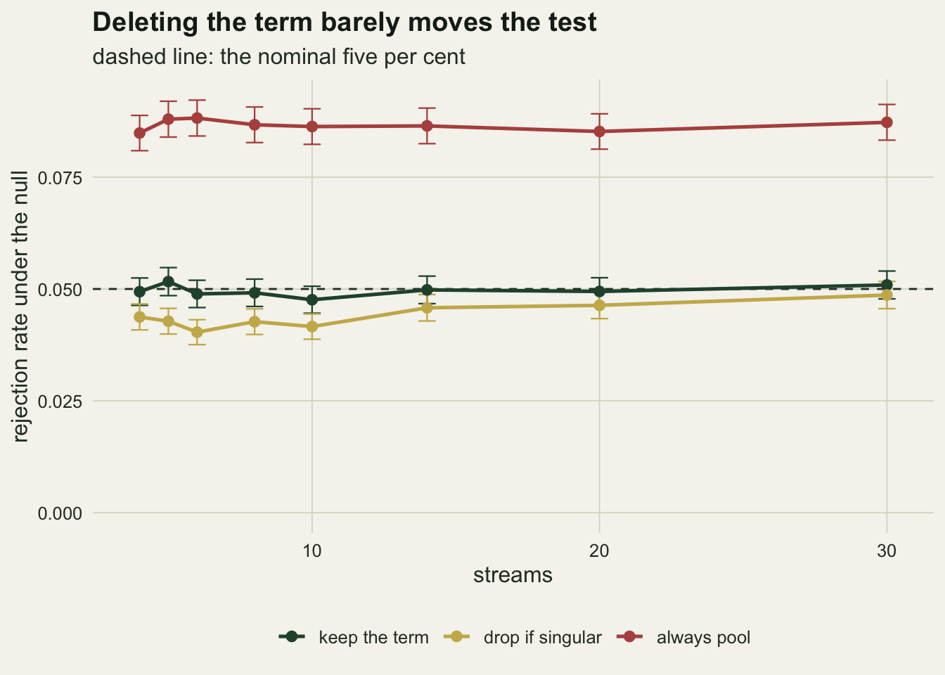
The unconditional rate hides two very different states
A five per cent rejection rate averaged over all datasets is not a five per cent rate in the dataset on the desk. Split the same 20000 replicates by whether the fit was singular and the average comes apart.
n_sing <- sum(pm$zero); n_ok <- sum(!pm$zero)
keep_sing <- mean(pm$keep[pm$zero]);  keep_ok <- mean(pm$keep[!pm$zero])
pool_sing <- mean(pm$pool[pm$zero]);  pool_ok <- mean(pm$pool[!pm$zero])
n_rej_ok <- sum(pm$keep[!pm$zero]); share_sing <- sum(pm$keep[pm$zero]) / sum(pm$keep)

n_grid <- c(2, 4, 8, 16, 32, 64)
set.seed(9127)
nsweep <- do.call(rbind, lapply(n_grid, function(nn) {
  pp <- procs(sim_fast(n_rep, n_strm, nn, 0, v_a, v_e))
  data.frame(n_per = nn, procedure = proc_lev, zero = mean(pp$zero),
             rate = c(mean(pp$keep), mean(pp$adapt), mean(pp$pool)))
}))
nsweep$procedure <- factor(nsweep$procedure, levels = proc_lev)
sw <- function(nn, k) nsweep$rate[nsweep$n_per == nn & nsweep$procedure == proc_lev[k]]
a_sub <- nsweep[nsweep$procedure == proc_lev[2], ]
a_max <- max(a_sub$rate); a_max_n <- a_sub$n_per[which.max(a_sub$rate)]
z_n64 <- nsweep$zero[nsweep$n_per == 64][1]; alt_b <- c(slope_set, -0.3, -0.5)
a_cross <- min(a_sub$n_per[a_sub$rate > alpha_lev])
a_dev <- max(abs(a_sub$rate[a_sub$n_per >= a_cross] - alpha_lev))
set.seed(7742)
share_alt <- vapply(alt_b, function(b) {
  pa <- procs(sim_fast(n_rep, n_strm, n_per, b, v_a, v_e), slope_true = b)
  c(sum(pa$keep[pa$zero]) / sum(pa$keep), mean(pa$keep))
}, numeric(2))
Among the 8713 singular datasets the correct test rejects 10.8 per cent of the time, more than twice its nominal rate. Among the 11287 datasets that returned a positive variance it rejects 0.27 per cent of the time: 30 rejections in total. So 96.9 per cent of the rejections this design produces under the null come from datasets in which the software would have printed a singular fit warning.
That matters more than the type I rate. The exact five per cent is an average of a state that rejects at twice the nominal level and a state that almost never rejects. The split survives under a real effect, but it loosens as the effect grows. At the generating slope of -0.12 the singular datasets still supply 87.1 per cent of the rejections; strengthen the slope to -0.3 and the share falls to 62.1 per cent, and at -0.5 to 45.1 per cent, by which point the test has 94 per cent power and no longer depends on a lucky draw. A singular fit is not a defect to clear before the analysis starts; at five streams it is the state in which a weak signal has most of its chance of showing up, and under the null nearly every rejection arrives with that warning attached. A strong signal does not need it.
The other thing worth varying is riffle effort, which is the direction effort usually goes when the streams are fixed.
cond <- data.frame(
  state = factor(rep(c("singular fit", "positive estimate"), each = 2),
                 levels = c("singular fit", "positive estimate")),
  procedure = factor(rep(proc_lev[c(1, 3)], 2), levels = proc_lev[c(1, 3)]),
  rate = c(keep_sing, pool_sing, keep_ok, pool_ok))

p_cond <- ggplot(cond, aes(state, rate, fill = procedure)) +
  geom_col(position = position_dodge(width = 0.7), width = 0.6,
           colour = te_paper, linewidth = 0.3) +
  geom_hline(yintercept = alpha_lev, colour = te_body, linetype = "dashed",
             linewidth = 0.5) +
  scale_fill_manual(values = c(te_forest, te_rust), name = NULL) +
  labs(x = NULL, y = "rejection rate under the null",
       title = "Five streams, split by state",
       subtitle = "green: keep the term, rust: pooling") +
  theme_datasheet() + theme(legend.position = "none")

p_sweep <- ggplot(nsweep, aes(n_per, rate, colour = procedure)) +
  geom_hline(yintercept = alpha_lev, colour = te_body, linetype = "dashed",
             linewidth = 0.5) +
  geom_line(linewidth = 0.9) + geom_point(size = 2.2) +
  scale_x_log10(breaks = n_grid) +
  scale_colour_manual(values = c(te_forest, te_gold, te_rust), name = NULL) +
  scale_y_continuous(limits = c(0, NA)) +
  guides(colour = guide_legend(nrow = 2)) +
  labs(x = "riffle samples per stream", y = "rejection rate under the null",
       title = "Five streams, more riffles",
       subtitle = "pooling explodes, the reflex does not") +
  theme_datasheet() + theme(legend.position = "bottom")

p_cond + p_sweep + plot_annotation(theme = theme_datasheet())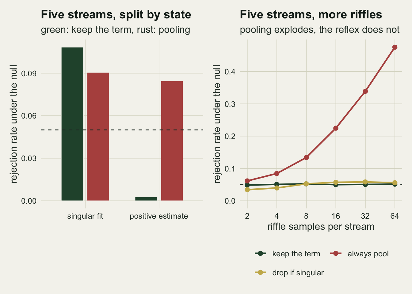
Holding the streams at five and raising the samples per stream, the reflex rejects 3.4 per cent at two samples, 4.0 per cent at four, peaks at 5.8 per cent at 32 samples and settles at 5.6 per cent at sixty four. It starts conservative and crosses the nominal line at 8 samples per stream; from there on it stays within 0.8 percentage points of nominal. The pooled test over the same range goes from 6.1 per cent to 47.5 per cent. The boundary rate at the largest design is still 5.3 per cent, so the rule is still firing; it has simply stopped protecting anything.
The interval carries the same message
Each procedure inverts its own test, so its coverage of the true slope is one minus its rejection rate by construction, and the coverage figures below carry nothing the previous section did not already have. The width does.
set.seed(4459)
pc <- procs(sim_fast(n_rep, n_strm, n_per, slope_set, v_a, v_e), slope_true = slope_set)
cov_keep <- mean(pc$cov_keep); cov_adapt <- mean(pc$cov_adapt); cov_pool <- mean(pc$cov_pool)
w_keep <- mean(pc$w_keep); w_adapt <- mean(pc$w_adapt); w_pool <- mean(pc$w_pool)
w_ratio_pool <- w_pool / w_keep; w_ratio_adapt <- w_adapt / w_keep; w_over_slope <- w_keep / abs(slope_set)
Over 20000 datasets generated with a real slope of -0.12, the interval that keeps the stream term covers 95.2 per cent of the time, the reflex 95.9 per cent and the fully pooled interval 91.3 per cent, with a Monte Carlo standard error of 0.2 percentage points. The mean widths are 0.528, 0.516 and 0.321 log units per ten percentage points logged. The pooled interval is 39 per cent narrower than the correct one and pays for that in coverage; the reflex is 2 per cent narrower and keeps its coverage.
The correct interval is wide. At five streams the 95 per cent interval spans 0.528 log units, 4.4 times the generating slope, and no choice of analysis fixes that. Barr and colleagues 2013 argue for keeping the random effects structure maximal on exactly these grounds, that removing a term buys apparent precision by testing against the wrong error term; Matuschek and colleagues 2017 reply that the maximal structure costs power when the term is genuinely near zero. The measurements here sit between them: for this design the deletion does little harm to the error rate, and the wide interval is the correct report for five streams either way.
What to report
Give the number of levels of the grouping factor before anything else. It sets the degrees of freedom of every test of a group level covariate, and at five levels it is the only number a reader needs in order to know how much the study can say.
Report the variance component that was estimated, including when it came out as zero, and call zero a boundary rather than a failed fit. A reader who knows the design can work out that a zero was the most likely single outcome, and describing it otherwise turns an ordinary draw into a mysterious computational problem.
If the fit was singular and the random term was deleted, say so, and say what happened to the degrees of freedom. The results here suggest the deletion is not the disaster it is usually called, for a balanced design with a group level covariate and few samples per group, but it is a data dependent choice, and a data dependent choice that is not reported cannot be checked.
Do not report a pooled analysis that never had a group term in it. That is the procedure that fails, at every design measured here, and it fails harder the more samples there are per group. The pooled test is not a simpler version of the mixed model; it is a test of a different null.
For a balanced design with a covariate constant within groups, consider reporting the regression on the group means as the primary analysis. Same slope, correct standard error, exact degrees of freedom, no fitting algorithm and no boundary to fall on. At five streams it is five numbers and one line of code, and it is the reference everything above was measured against.
Honest limits
Everything here is a balanced Gaussian one way design with the covariate constant within a group. That is the case where the moment estimator is closed form and the group means analysis is exact, and it is why no mixed model fitting software appears anywhere in this post. Unbalanced groups, crossed grouping factors, random slopes and non Gaussian responses all break the closed form, and there is no reason to expect the near balance that keeps the reflex calibrated here to survive any of them. The result to carry forward is the conditional split, not the type I rate.
The covariate also sits at the group level throughout. A covariate that varies within groups is tested against a different error term, and the effect of deleting the random intercept on that test is a separate question with a different answer, which is part of why the folklore about singular fits is so mixed.
The generating intraclass correlation is fixed at 0.10. That is a low but not unusual value for stream invertebrate biomass. A larger one lowers the boundary rate and makes pooling worse; a value of exactly zero raises the boundary rate above one half and makes the pooled test exactly valid, for the accidental reason that there is then nothing to pool over. None of the numbers here should be read as design advice for a different intraclass correlation without rerunning the code.
The decision rule tested is the crisp one: the estimate is exactly zero, so the term goes. Real analysis is fuzzier. People delete terms on near zero estimates, on convergence warnings, on likelihood ratio tests against a nominal chi squared, and sometimes after seeing the p value they wanted. Each is a different rule with its own error rate, and a rule that peeks at the outcome will be worse than anything measured here.
Finally, this post measures a decision rule, not an estimator. Stram and Lee 1994 and Self and Liang 1987 give the asymptotic distribution of the likelihood ratio statistic when the null sits on a boundary, which is the tool for testing whether a variance component is zero. Nothing above tests that hypothesis, because in this design the answer is already known and the interesting question is what the analyst does next.
References
Stram DO, Lee JW 1994 Biometrics 50(4):1171 (10.2307/2533455)
Self SG, Liang KY 1987 Journal of the American Statistical Association 82(398):605-610 (10.1080/01621459.1987.10478472)
Bates D, Machler M, Bolker B, Walker S 2015 Journal of Statistical Software 67(1) (10.18637/jss.v067.i01)
Barr DJ, Levy R, Scheepers C, Tily HJ 2013 Journal of Memory and Language 68(3):255-278 (10.1016/j.jml.2012.11.001)
Matuschek H, Kliegl R, Vasishth S, Baayen H, Bates D 2017 Journal of Memory and Language 94:305-315 (10.1016/j.jml.2017.01.001)
Gelman A, Hill J 2007 Data Analysis Using Regression and Multilevel/Hierarchical Models (ISBN 978-0-521-68689-1)