The parametric bootstrap and a boundary problem

Simulate from a fitted model to build a null distribution the asymptotic chi-squared gets wrong, and test Poisson against negative binomial overdispersion honestly.

The previous post resampled the data. The parametric bootstrap resamples from a model instead: fit the model you believe holds under the null hypothesis, simulate fresh datasets from it, and recompute your statistic on each. The spread of those simulated statistics is the null distribution you need. This is the right tool when the data-resampling bootstrap does not apply, and above all when a textbook asymptotic distribution is quietly wrong.

A common ecological case where the textbook answer is wrong: testing whether count data are overdispersed. We fit a Poisson generalised linear model and a negative binomial alternative, and compare them with a likelihood-ratio test. The trouble is that Poisson is negative binomial with the dispersion pushed to its limit, and that limit sits on the boundary of the parameter space. When a null value lies on a boundary, the likelihood-ratio statistic does not follow the chi-squared distribution everyone reaches for. The parametric bootstrap fixes it without any special theory.

Why the chi-squared is wrong here

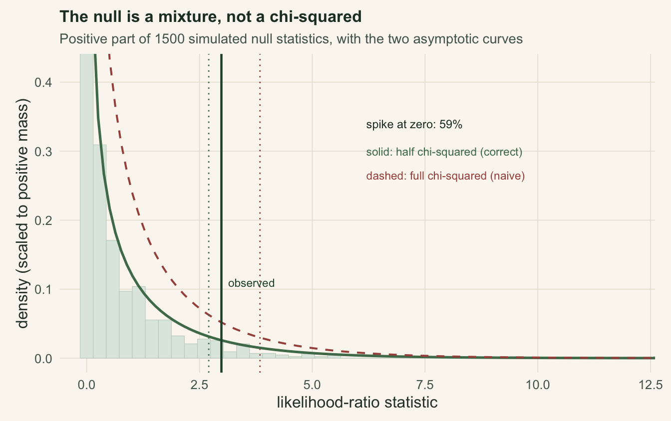
The negative binomial has a dispersion parameter; write it so that the Poisson corresponds to one over that parameter being zero. Poisson is the negative binomial with the extra variance switched off. That zero is the smallest value the parameter can take, so under the null the truth sits at the edge of the allowed range. Standard likelihood theory assumes the null value is in the interior, with wiggle room on both sides. On a boundary that assumption fails, and the likelihood-ratio statistic no longer has an asymptotic chi-squared distribution on one degree of freedom. The correct large-sample answer is a fifty-fifty mixture of a point mass at zero and a chi-squared on one degree of freedom. Half the time the fitted dispersion wants to go negative, is held at zero, and the statistic is exactly zero.

Using the naive chi-squared ignores that spike at zero, so it places its critical value too far out and rejects too rarely. In overdispersion terms: the naive test is conservative and will tell you to keep Poisson when you should not.

Overdispersed counts along a gradient

We simulate abundance counts with modest overdispersion along an environmental gradient, then fit both models.

set.seed(243)
n <- 90
x <- as.numeric(scale(runif(n, 0, 10)))     # standardised environmental gradient
mu <- exp(1.15 + 0.5 * x)
y <- rnbinom(n, size = 6, mu = mu)           # counts with mild overdispersion
disp_obs <- var(y) / mean(y)                 # crude variance-to-mean ratio

The counts have a variance-to-mean ratio of 2.13, a hint of extra spread but nothing dramatic. The question is whether that hint is real or noise.

The likelihood-ratio statistic and its wrong p-value

The statistic is twice the gain in log-likelihood from Poisson to negative binomial. We clamp it at zero, since the negative binomial can never fit worse than the Poisson it contains.

lrt_stat <- function(y, x) {
  m_pois <- glm(y ~ x, family = poisson)
  m_nb <- suppressWarnings(tryCatch(glm.nb(y ~ x), error = function(e) NULL))
  if (is.null(m_nb)) return(0)
  max(0, 2 * (as.numeric(logLik(m_nb)) - as.numeric(logLik(m_pois))))
}
LRT_obs <- lrt_stat(y, x)
p_naive <- 1 - pchisq(LRT_obs, df = 1)         # naive chi-squared(1)
p_mix   <- 0.5 * (1 - pchisq(LRT_obs, df = 1)) # asymptotic 50:50 mixture

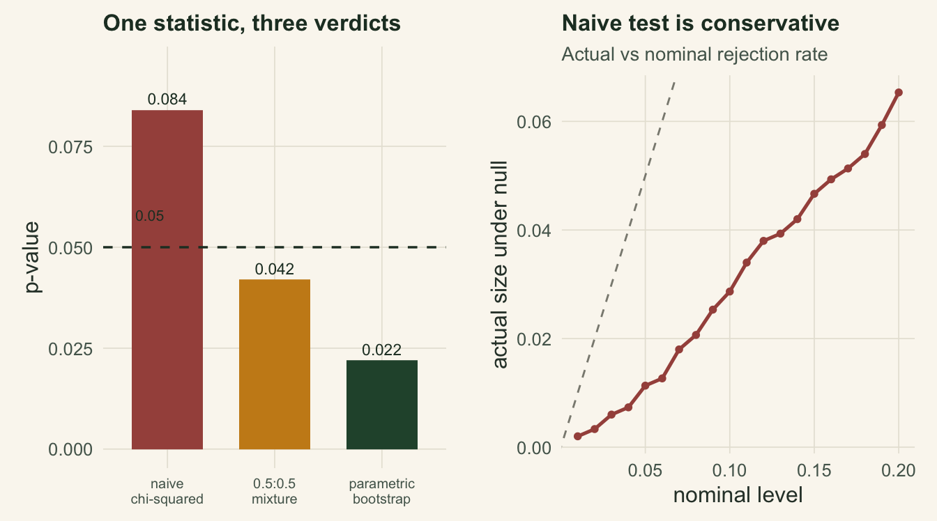
The observed statistic is 2.99. Fed through the naive chi-squared on one degree of freedom it gives a p-value of 0.084, comfortably above 0.05: the naive test says there is no overdispersion, keep Poisson. The boundary-aware mixture halves that to 0.042, which is below 0.05. Same statistic, opposite conclusion. The naive p-value is exactly twice the mixture one, because it forgets that half the null mass sits at zero.

The parametric bootstrap null

Rather than trust either asymptotic formula, we build the null distribution directly. Under the null the data are Poisson, so we simulate from the fitted Poisson model, refit both models to each simulated dataset, and collect the likelihood-ratio statistics.

m_pois <- glm(y ~ x, family = poisson)
mu_hat <- fitted(m_pois)
set.seed(909)
Bpb <- 1500
LRT_star <- replicate(Bpb, lrt_stat(rpois(n, mu_hat), x))
p_boot <- (1 + sum(LRT_star >= LRT_obs)) / (Bpb + 1)
frac0  <- mean(LRT_star < 1e-6)                # share of the null exactly at zero

The parametric bootstrap p-value is 0.022, agreeing with the mixture that the overdispersion is real, and if anything more decisive. It also shows why the boundary matters: 59% of the simulated null statistics are exactly zero, a point mass the chi-squared curve has no way to represent. That fraction is even a little above the asymptotic fifty percent, because in samples this size the fitted dispersion is pulled to the boundary slightly more than half the time.

Figure 1: The parametric bootstrap null distribution of the likelihood-ratio statistic (1500 simulations from the fitted Poisson). A large share of the null is a spike at zero (annotated), and the positive part follows half a chi-squared on one degree of freedom (solid), not the full chi-squared the naive test assumes (dashed), which sits too high and so overstates the tail. The observed statistic (vertical line) lies beyond the mixture critical value but short of the naive one.

The naive test is conservative

Because the simulated statistics come from the null, they let us read off the naive test’s real error rate. A test with a nominal five percent level should reject five percent of the time when the null holds.

naive_size <- mean(LRT_star > qchisq(0.95, 1))   # actual size of the naive 5% test
alpha_grid <- seq(0.01, 0.20, by = 0.01)
size_naive <- sapply(alpha_grid, function(a) mean(LRT_star > qchisq(1 - a, 1)))

At its nominal five percent, the naive chi-squared test actually rejects only 1.1% of the time under the null: it throws away most of its power to detect overdispersion in exchange for a false sense of caution. The parametric bootstrap, by using the correct null quantiles, hits the nominal level by construction.

Figure 2: Left: the three p-values for the observed test. The naive chi-squared sits above 0.05 (keep Poisson) while the mixture and the parametric bootstrap sit below it (adopt the negative binomial). Right: the naive test’s actual rejection rate under the null against its nominal level; the curve stays below the diagonal everywhere, so the naive test is uniformly conservative. The parametric bootstrap lies on the diagonal by construction.

What to take away

The parametric bootstrap earns its place whenever you can simulate from the model under the null but cannot trust the asymptotic reference distribution. Boundary parameters are the classic trap: testing a variance component against zero, testing overdispersion, testing a mixture component, all put the null value on an edge, and all break the usual chi-squared. Simulating from the fitted null model sidesteps the theory and gives the right p-value, here rescuing a real overdispersion signal that the naive test would have dismissed. The cost is that the parametric bootstrap trusts the null model completely: if the Poisson mean structure is itself misspecified, simulating from it inherits that error. Resample from the model you are willing to defend, and the next post shows what goes wrong when even the data-resampling bootstrap is applied to data that are not independent.

Related tutorials

• The nonparametric bootstrap
• Bootstrapping dependent data
• Checking a bootstrap
• Count data and abundance GLMs

References

Efron 1979 Annals of Statistics 7(1):1-26 (10.1214/aos/1176344552)

Self and Liang 1987 Journal of the American Statistical Association 82(398):605-610 (10.1080/01621459.1987.10478472)

DiCiccio and Efron 1996 Statistical Science 11(3):189-228 (10.1214/ss/1032280214)

Davison and Hinkley 1997 Bootstrap Methods and their Application. ISBN 978-0-521-57391-7

Manly 2007 Randomization, Bootstrap and Monte Carlo Methods in Biology, third edition. ISBN 978-1-58488-541-2