---
title: "Revisit designs for long-term monitoring"
description: "Four revisit schedules on one annual budget in R: re-using sites sharpens the trend and blurs the regional mean, and the design enters through one matrix."
date: "2026-06-26 10:00"
categories: [R, survey design, monitoring, ecology tutorial]
date-modified: "2026-09-27"
image: thumbnail.png
image-alt: "Scatter plot of four monitoring designs positioned by the standard error of their trend estimate against the standard error of their regional mean"
---
*Corrected 27 September 2026: the closing limits said the middle two designs could swap places under other variance components; under the model used here they cannot, since only the size of the gaps changes, and the text now says so. The schedule figure's caption also said every panel has the same number of filled cells in every year, which the cropped drawing does not show; it now says this holds for the full pool only.*
A monitoring programme can afford a fixed number of site visits per year. The number is set by staff and money, and it rarely changes. What does change, and what is nearly free to change, is which sites those visits go to: the same ones every year, a fresh set every year, or something in between.
That choice is the revisit design. It is usually made once, at the start, without measurement. This post spends the same annual budget four different ways over the same twelve years, and works out exactly what each one delivers.
## Four ways to spend the same budget
Thirty site visits a year, twelve years, two counts per visit. Every design below costs exactly the same.
```{r designs}
n_visit <- 30      # site visits per year
n_year  <- 12
n_rep   <- 2       # counts per site visit

# a design maps each year to the site identifiers visited that year
visits <- function(design) {
  switch(design,
    always = lapply(1:n_year, function(j) 1:n_visit),
    rotate = lapply(1:n_year, function(j) ((j - 1) %% 4) * n_visit + 1:n_visit),
    split  = lapply(1:n_year, function(j) c(1:15, 15 + ((j - 1) %% 4) * 15 + 1:15)),
    fresh  = lapply(1:n_year, function(j) (j - 1) * n_visit + 1:n_visit))
}
designs <- c("always", "rotate", "split", "fresh")
distinct <- sapply(designs, function(d) length(unique(unlist(visits(d)))))
data.frame(design = designs, distinct_sites = unname(distinct),
           visits_per_site = round(n_visit * n_year / unname(distinct), 1))
```
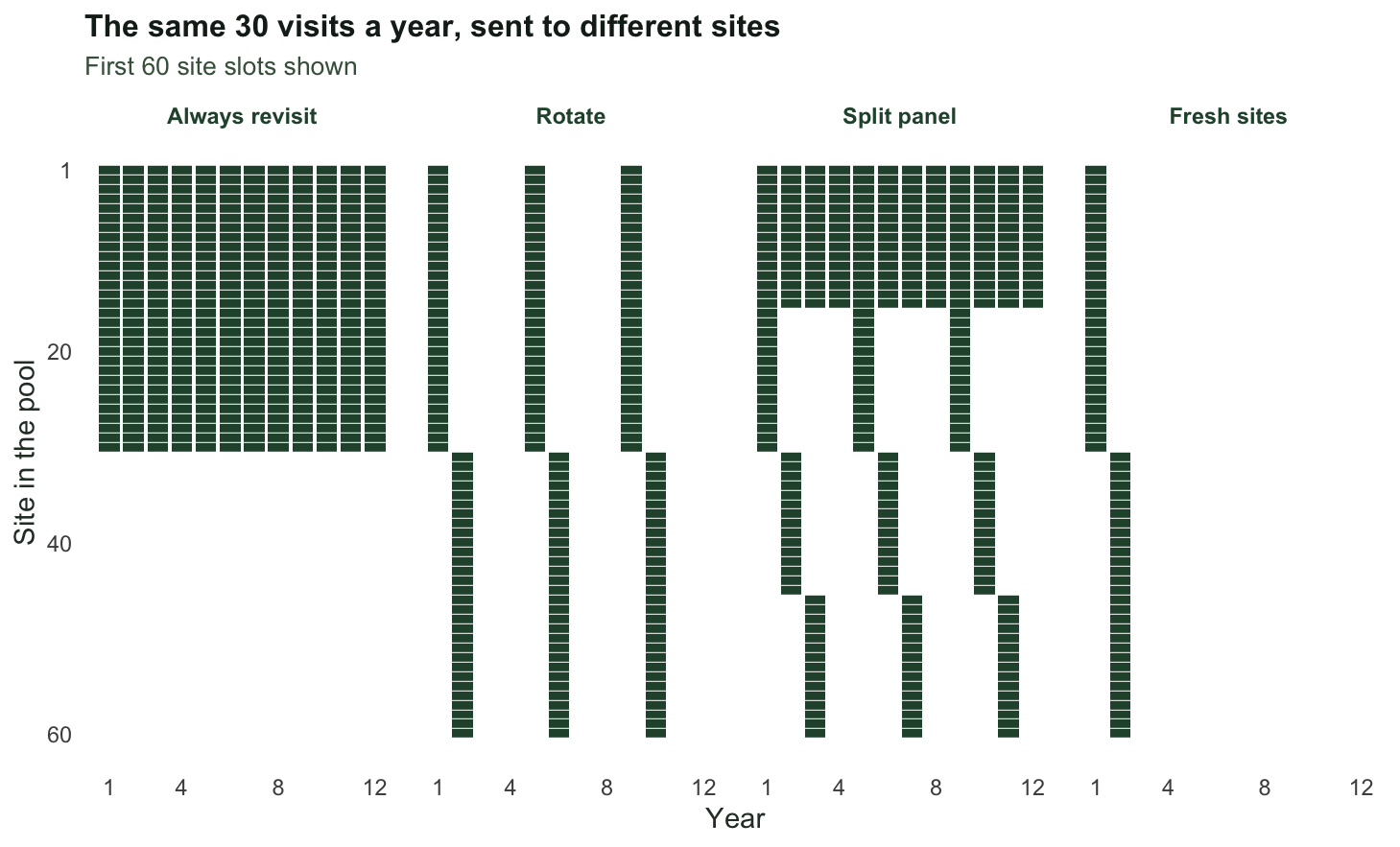
**Always revisit** keeps 30 permanent sites and returns to all of them every year. **Rotate** holds 120 sites in four panels of 30 and works through them on a four year cycle, so each site is seen three times in twelve years. **Split** keeps 15 permanent sites and rotates the other 15 visits through four panels of 15. **Fresh** draws 30 new sites every year and never returns.
```{r fig-schedule}
#| echo: false
#| fig-width: 7.6
#| fig-height: 4.6
#| fig-cap: "Visit schedules for the four designs. Each row is a site in the pool and each column a year; a filled cell is a visit. Only the first 60 site slots are drawn, so the fresh design shows just its first two annual blocks. In the full pool every design makes 30 visits in every year; the cropped view hides the rest."
#| fig-alt: "Four small grids side by side showing which site is visited in which year: a solid block for always revisit, a repeating diagonal for rotate, a solid strip plus a diagonal for split, and a single staircase for fresh sites."
library(ggplot2)
theme_te <- function(base_size = 11) {
theme_minimal(base_size = base_size) +
theme(plot.background = element_rect(fill = "#f5f4ee", colour = NA),
panel.background = element_rect(fill = "#f5f4ee", colour = NA),
panel.grid = element_blank(),
text = element_text(colour = "#2c3a31"),
plot.title = element_text(colour = "#16241d", face = "bold", size = base_size + 1),
plot.subtitle = element_text(colour = "#46604a", size = base_size - 1),
strip.text = element_text(colour = "#275139", face = "bold"))
}
grid_df <- do.call(rbind, lapply(designs, function(dn) {
v <- visits(dn)
do.call(rbind, lapply(1:n_year, function(j) {
ids <- v[[j]]; ids <- ids[ids <= 60]
if (length(ids) == 0) NULL else data.frame(design = dn, year = j, site = ids)
}))
}))
grid_df$design <- factor(grid_df$design, levels = designs,
labels = c("Always revisit", "Rotate", "Split panel", "Fresh sites"))
ggplot(grid_df, aes(year, site)) +
geom_tile(fill = "#275139", width = 0.85, height = 0.9) +
facet_wrap(~design, nrow = 1) +
scale_x_continuous(breaks = c(1, 4, 8, 12)) +
scale_y_reverse(breaks = c(1, 20, 40, 60)) +
labs(x = "Year", y = "Site in the pool",
title = "The same 30 visits a year, sent to different sites",
subtitle = "First 60 site slots shown") +
theme_te()
```
## The design enters through one matrix
The data model is the one from the previous post: a persistent site level, a year effect shared by every site, a site by year interaction, and counting noise on each visit. Both headline numbers come from the annual means, so the whole comparison reduces to the covariance matrix of those `r n_year` numbers.
Two years share a year effect only if they are the same year. They share site levels in proportion to how many sites they have in common. Write that overlap count as `O[j, j']`, and the covariance of the annual means is
```{r covariance}
sd_site <- 0.55; sd_year <- 0.20; sd_sy <- 0.30; sd_res <- 0.35
beta_true <- -0.03
tc  <- (1:n_year) - mean(1:n_year)
Sxx <- sum(tc^2)

overlap <- function(v) {
  outer(1:n_year, 1:n_year, Vectorize(function(i, j) length(intersect(v[[i]], v[[j]]))))
}
cov_annual <- function(v) {
  within_year <- sd_year^2 + (sd_sy^2 + sd_res^2 / n_rep) / n_visit
  diag(n_year) * within_year + sd_site^2 * overlap(v) / n_visit^2
}
overlap(visits("split"))[1:5, 1:5]
```
The split panel shares 15 sites between any two years and all 30 when the years are four apart. That single matrix carries the entire design.
The slope from a regression of the annual means on year is a fixed linear combination of them, with weights `w = (t - tbar) / Sxx` that sum to zero. The period mean uses equal weights. So both variances are quadratic forms, and no simulation is needed.
```{r exact-variances}
w_trend  <- tc / Sxx
w_status <- rep(1 / n_year, n_year)

exact <- t(sapply(designs, function(d) {
  S <- cov_annual(visits(d))
  c(se_trend  = sqrt(drop(t(w_trend)  %*% S %*% w_trend)),
    se_status = sqrt(drop(t(w_status) %*% S %*% w_status)))
}))
exact <- data.frame(design = designs, distinct = unname(distinct), exact,
                    trend_rel  = exact[, "se_trend"]  / exact[1, "se_trend"],
                    status_rel = exact[, "se_status"] / exact[1, "se_status"])
print(exact, digits = 4, row.names = FALSE)
```
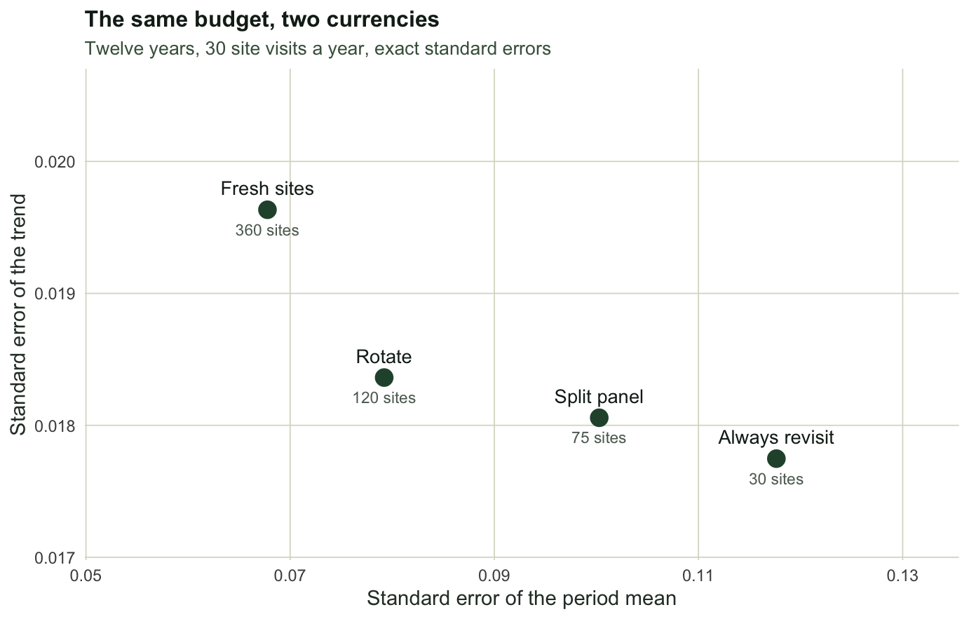
Every design gives an unbiased slope, so the table is a comparison of precision alone, and the two columns move in opposite directions.
```{r mc-check}
set.seed(368)
run_design <- function(design, B = 3000) {
  v <- visits(design); npool <- length(unique(unlist(v)))
  t(replicate(B, {
    s <- rnorm(npool, 0, sd_site)
    a <- rnorm(n_year, 0, sd_year)
    annual <- vapply(1:n_year, function(j) {
      ids <- v[[j]]
      mean(3 + beta_true * tc[j] + s[ids] + a[j] +
           rnorm(length(ids), 0, sd_sy) + rnorm(length(ids), 0, sd_res / sqrt(n_rep)))
    }, numeric(1))
    c(slope = unname(coef(lm(annual ~ tc))[2]), status = mean(annual))
  }))
}
mc <- t(sapply(designs, function(d) {
  m <- run_design(d)
  c(mc_trend = sd(m[, "slope"]), mc_status = sd(m[, "status"]),
    bias = mean(m[, "slope"]) - beta_true)
}))
round(cbind(mc, exact_trend = exact$se_trend, exact_status = exact$se_status), 5)
```
Simulation reproduces the exact values, and the largest bias across `r format(4 * 3000, big.mark = ",")` simulated programmes is `r sprintf("%.5f", max(abs(mc[, "bias"])))` against a true slope of `r beta_true`. From here the exact numbers are used, because they carry no Monte Carlo error at all.
```{r fig-tradeoff}
#| echo: false
#| fig-width: 7.2
#| fig-height: 4.6
#| fig-cap: "Each design plotted by what it delivers. Left is a sharper regional mean, down is a sharper trend. Nothing sits in the bottom left corner: re-using sites moves a programme down and to the right, and the rotating panel sits nearest that empty corner."
#| fig-alt: "Scatter plot with four labelled points forming an arc from the top left to the bottom right, showing the trade-off between precision of the regional mean and precision of the trend."
pl <- data.frame(x = exact$se_status, y = exact$se_trend,
lab = c("Always revisit", "Rotate", "Split panel", "Fresh sites"),
sub = paste0(exact$distinct, " sites"))
ggplot(pl, aes(x, y)) +
geom_point(colour = "#275139", size = 4) +
geom_text(aes(label = lab), vjust = -1.1, colour = "#16241d", size = 3.6) +
geom_text(aes(label = sub), vjust = 2.2, colour = "#5d6b61", size = 3) +
expand_limits(x = range(pl$x) + c(-0.014, 0.014),
y = range(pl$y) + c(-0.0006, 0.0009)) +
labs(x = "Standard error of the period mean",
y = "Standard error of the trend",
title = "The same budget, two currencies",
subtitle = "Twelve years, 30 site visits a year, exact standard errors") +
theme_te() +
theme(panel.grid.major = element_line(colour = "#dad9ca", linewidth = 0.3))
```
## Why re-use helps one and hurts the other
Both effects come out of the quadratic forms, and they land on the overlap matrix from opposite sides.
The trend weights sum to zero. If two years share the same number of sites no matter which two years they are, the site term is the same constant everywhere in the matrix, and a constant added to every entry contributes nothing to a contrast. That is exactly the always-revisit design, and its site contribution is zero up to floating-point rounding. Any design in which the overlap depends on the year gap leaves a residue, and that residue is a cost.
```{r fp-guard-1}
#| include: false
stopifnot(abs(drop(t(w_trend) %*% overlap(visits("always")) %*% w_trend)) <
1e-8 * abs(drop(t(w_trend) %*% overlap(visits("fresh")) %*% w_trend)))
```
The period mean weights are all positive, so the site term enters through the total of the overlap matrix. That total is what an effective number of sites means.
```{r effective-sites}
eff_sites <- sapply(designs, function(d) {
  O <- overlap(visits(d))
  n_visit^2 * n_year^2 / sum(O)
})
data.frame(design = designs, distinct_sites = unname(distinct),
           effective_sites = round(unname(eff_sites), 1))
```
The split panel visits `r distinct[["split"]]` distinct sites but is worth only `r sprintf("%.0f", eff_sites[["split"]])` of them for the regional mean, because its permanent half is counted twelve times and its rotating half three times. Distinct sites are not the currency; the total of the overlap matrix is.
## How large is the penalty
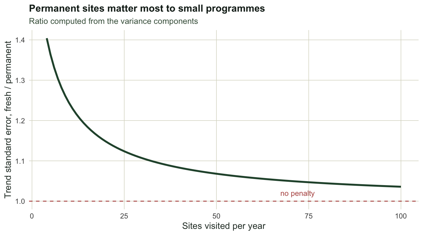
The trend cost of never returning depends on how many sites are visited each year, because the site component enters the annual mean divided by that number.
```{r penalty-curve}
penalty <- function(n) {
  base <- sd_year^2 + (sd_sy^2 + sd_res^2 / n_rep) / n
  sqrt((base + sd_site^2 / n) / base)
}
data.frame(sites_per_year = c(5, 10, 20, 30, 60, 100),
           trend_se_penalty = round(penalty(c(5, 10, 20, 30, 60, 100)), 3))
```
```{r fig-penalty}
#| echo: false
#| fig-width: 7.2
#| fig-height: 4.0
#| fig-cap: "Cost of never returning to a site, as a function of how many sites are visited each year. The penalty is the ratio of trend standard errors, fresh sites against permanent sites. It is large for a small programme and close to nothing for a large one."
#| fig-alt: "Decreasing curve starting near 1.40 at four sites per year and flattening towards 1.04 by one hundred sites per year, with a dashed reference line at one."
nseq <- seq(4, 100, by = 1)
ggplot(data.frame(n = nseq, p = penalty(nseq)), aes(n, p)) +
geom_hline(yintercept = 1, linetype = "dashed", colour = "#b5534e") +
geom_line(colour = "#275139", linewidth = 1.1) +
annotate("text", x = 72, y = 1.02, label = "no penalty", colour = "#b5534e", size = 3.2) +
labs(x = "Sites visited per year", y = "Trend standard error, fresh / permanent",
title = "Permanent sites matter most to small programmes",
subtitle = "Ratio computed from the variance components") +
theme_te() +
theme(panel.grid.major = element_line(colour = "#dad9ca", linewidth = 0.3))
```
At five sites a year the penalty for never returning is `r sprintf("%.2f", penalty(5))`, and at one hundred it is `r sprintf("%.2f", penalty(100))`. The rule that permanent sites protect a trend is real, and it matters most to the smallest programmes.
Rotating is far cheaper than never returning, and the reason is visible in the exact table: a four year cycle costs `r sprintf("%.1f", 100 * (exact$trend_rel[2] - 1))` per cent on the trend against the `r sprintf("%.1f", 100 * (exact$trend_rel[4] - 1))` per cent of a fresh sample, because every site does come back twice more and part of the cancellation is recovered. The split panel costs `r sprintf("%.1f", 100 * (exact$trend_rel[3] - 1))` per cent on the trend and saves `r sprintf("%.0f", 100 * (1 - exact$status_rel[3]))` per cent on the regional mean, which is why it is the standard recommendation in the monitoring literature.
The honest limit is that every number here came out of one set of variance components. Change the ratio of site variance to year variance and the gaps between the designs grow or shrink, but under this model their order in each column does not change: the site variance scales every design's overlap term by the same factor, and the rest of the variance is common to all four. A programme should estimate its own components first and re-run the table with them, which means changing four numbers in the code above.
There is also a question this post has not asked: whether the sites in the pool represent the region at all. A design can be excellent for trend and describe nothing, if the sites were chosen because they were easy to reach.
## Where this leaves the series
The design fixes the standard error. Whether that standard error is small enough to answer the question is a separate calculation, and it is the one most programmes skip. The next post does it.
## References
Urquhart, Paulsen and Larsen 1998 Ecological Applications 8(2):246-257 (10.1890/1051-0761(1998)008[0246:MFPRRO]2.0.CO;2)
Urquhart and Kincaid 1999 Journal of Agricultural, Biological, and Environmental Statistics 4(4):404-414 (10.2307/1400498)
Larsen, Kincaid, Jacobs and Urquhart 2001 BioScience 51(12):1069-1078 (10.1641/0006-3568(2001)051[1069:DFELAR]2.0.CO;2)
Rhodes and Jonzen 2011 Ecography 34(6):1040-1048 (10.1111/j.1600-0587.2011.06370.x)
## Related tutorials
- [Variance components in monitoring data](../variance-components-in-monitoring/)
- [Power to detect a population trend](../power-to-detect-a-population-trend/)
- [Checking a monitoring design](../checking-a-monitoring-design/)
- [When to stop monitoring](../when-to-stop-monitoring/)