library(ggplot2)

te_pal <- list(forest = "#275139", green = "#2f8f63", sage = "#93a87f",
               clay = "#b5534e", gold = "#cda23f", line = "#dad9ca",
               ink = "#16241d", paper = "#f5f4ee")

theme_te <- function() {
  theme_minimal(base_size = 12) +
    theme(panel.grid.minor = element_blank(),
          panel.grid.major = element_line(colour = "#e7e6dc"),
          plot.background = element_rect(fill = "#f5f4ee", colour = NA),
          panel.background = element_rect(fill = "#f5f4ee", colour = NA),
          plot.title = element_text(face = "bold", colour = te_pal$ink),
          axis.title = element_text(colour = "#2c3a31"))
}When to stop monitoring
R
monitoring
decision analysis
ecology tutorial
ggplot2
Monitoring has a stopping rule. Backward induction in R prices a further year of survey against the cost of delay, and what waiting for a p-value costs.
A harbour authority has been surveying seagrass cover in a sheltered bay every August for nine years. Divers work the same fixed transects, the quadrats go into a spreadsheet, and the mean cover for the year gets a point on a graph that is passed round the estuary partnership in November. The graph slopes down. It slopes down by a fraction of a per cent a year, with a standard error several times the size of the slope, so the graph has been passed round for nine years without anybody being able to say from it whether the meadow is going or staying. The swinging moorings that are the suspected cause are still in the water, and replacing them with helical anchors would cost 260 thousand pounds. Somebody eventually asks the question that monitoring programmes almost never put in writing: how many more summers of this before we decide?
That question has an answer, and it is not a matter of custom. This tutorial writes the problem down as an optimal stopping problem: a belief about the trend that updates as each survey lands, a cost for putting the anchors in, a cost for leaving the moorings where they are if the meadow really is going, and a cost for every year spent deciding. Backward induction over that structure returns a rule rather than a recommendation, and the rule is then measured against the two that get used in practice, monitor for a round number of years and monitor until the trend test comes out significant. The second of those costs more than half the price of the works it is meant to justify.
The expected value of information prices a survey placed once, before a decision that is taken once: pay, learn, decide. The question here is sequential, because the decision comes back every autumn and the meadow keeps shrinking while it stays open, so today’s decision to wait changes the state that tomorrow’s decision faces. Power to detect a population trend sizes the same survey against a different criterion, the chance of a significant slope, and one of the measurements below is what that criterion is worth here.
A meadow, a mooring field and nine summers of data
The index is the mean per cent cover across the transects, and it is modelled on the log scale as a straight line in time plus survey error. The slope of that line is the annual rate of change and is the only unknown that matters here. The survey error has a standard deviation of 0.18 on the log scale, which is what a diver survey of this design delivers and is large enough that a single summer tells you very little.
Four numbers turn the ecology into a decision. Replacing the moorings costs 260 thousand pounds and is assumed to halt the decline outright. Each further summer of survey costs 9 thousand. The authority values the meadow at 700 thousand pounds per unit of annual log decline rate, which is its stated exchange rate between losing seagrass and spending money: a bed shrinking at one per cent a year is losing about 7 thousand pounds of value a year. The management horizon is 30 years. Those four are choices, not measurements, and the last section returns to that.
s_obs   <- 0.18
n_hist  <- 9
horizon <- 30
c_surv  <- 9
c_act   <- 260
d_loss  <- 700
k_max   <- 25
beta_true <- -0.014

round(c(survey_sd = s_obs, summers_done = n_hist, horizon_years = horizon,
        cost_per_survey = c_surv, cost_of_works = c_act,
        loss_per_unit_rate = d_loss, longest_extension = k_max,
        true_rate = beta_true), 4)
survey_sd summers_done horizon_years cost_per_survey
0.180 9.000 30.000 9.000
cost_of_works loss_per_unit_rate longest_extension true_rate
260.000 700.000 25.000 -0.014 sxx <- function(n) n * (n^2 - 1) / 12
post_var <- function(k, so = s_obs) so^2 / sxx(n_hist + k)
set.seed(20260723)
hist_yr <- 1:n_hist
y_hist <- log(38) + beta_true * hist_yr + rnorm(n_hist, 0, s_obs)
tb_h <- mean(hist_yr)
m0 <- sum((hist_yr - tb_h) * y_hist) / sxx(n_hist)
cbar <- mean(y_hist)
vk <- post_var(0:k_max)
print(round(exp(y_hist), 2))[1] 32.49 34.39 27.04 39.57 34.14 29.74 37.72 34.76 27.43round(c(true_rate_per_cent = 100 * (exp(beta_true) - 1),
fitted_rate = m0, per_cent_a_year = 100 * (exp(m0) - 1),
posterior_sd = sqrt(vk[1]),
prob_declining = pnorm(0, m0, sqrt(vk[1]))), 5)true_rate_per_cent fitted_rate per_cent_a_year posterior_sd
-1.39025 -0.00441 -0.44010 0.02324
prob_declining
0.57527 The nine summers are simulated from a true rate of decline of 1.39 per cent a year so that every rule below can be scored against a truth that is known. What those nine summers actually produce is a fitted rate of -0.00441, a decline of 0.44 per cent a year, with a standard error of 0.02324. The posterior probability that the meadow is declining at all is 0.57527. Nine years of careful diving have moved that probability barely off a coin toss, which is the situation the stopping rule has to work in and is not unusual for a seagrass programme.
The decision written down
Two functions are needed. The first says what the manager believes after any number of further summers, and the second says what it costs to stop believing and act.
With a flat prior on the intercept and on the slope, the posterior for the slope after \(n\) annual surveys is normal, centred on the least squares slope, with variance \(\sigma^2 / S_{xx}\) where \(S_{xx} = n(n^2-1)/12\) for equally spaced years. The variance does not depend on the data at all, only on how many years have been surveyed, so it is known in advance. That collapses the belief state to a single number, the posterior mean, and it makes the belief a martingale: the expected posterior mean next year is the posterior mean today, and the variance of the step is exactly the drop in posterior variance. Both facts are worth checking rather than taking on trust, because everything downstream depends on them.
step_sd <- sqrt(-diff(vk))
print(round(rbind(further_summers = 0:8, posterior_sd = sqrt(vk[1:9]),
                  step_sd = c(step_sd[1:8], NA)), 5))
[,1] [,2] [,3] [,4] [,5] [,6] [,7] [,8]
further_summers 0.00000 1.00000 2.00000 3.00000 4.00000 5.00000 6.00000 7.00000
posterior_sd 0.02324 0.01982 0.01716 0.01505 0.01334 0.01193 0.01076 0.00976
step_sd 0.01214 0.00991 0.00824 0.00697 0.00597 0.00517 0.00452 0.00399
[,9]
further_summers 8.00000
posterior_sd 0.00891
step_sd NAsim_fwd <- function(nrep, seed, proc_sd = 0, so_true = s_obs) {
set.seed(seed)
beta0 <- rnorm(nrep, m0, sqrt(vk[1]))
lev <- rnorm(nrep, cbar, s_obs / sqrt(n_hist))
now <- lev + beta0 * (n_hist - tb_h)
xx <- matrix(0, nrep, horizon + 1)
bt <- beta0
for (j in 1:horizon) {
if (proc_sd > 0) bt <- bt + rnorm(nrep, 0, proc_sd)
xx[, j + 1] <- xx[, j] + bt
}
Sy <- rep(sum(y_hist), nrep); Sty <- rep(sum(hist_yr * y_hist), nrep)
mm <- matrix(NA_real_, nrep, k_max + 1); mm[, 1] <- m0
for (k in 1:k_max) {
n <- n_hist + k
ynew <- now + xx[, k + 1] + rnorm(nrep, 0, so_true)
Sy <- Sy + ynew; Sty <- Sty + n * ynew
mm[, k + 1] <- (Sty - ((n + 1) / 2) * Sy) / sxx(n)
}
list(beta = beta0, mm = mm, xx = xx)
}
n_rep <- 30000
sm <- sim_fwd(n_rep, 20260723)
inc_var <- apply(diff(t(sm$mm)), 1, var)
print(round(rbind(simulated = inc_var[1:6], predicted = (-diff(vk))[1:6]), 8)) [,1] [,2] [,3] [,4] [,5] [,6]
simulated 0.00014710 9.781e-05 6.738e-05 4.848e-05 3.50e-05 2.653e-05
predicted 0.00014727 9.818e-05 6.797e-05 4.855e-05 3.56e-05 2.670e-05c(replicates = n_rep)replicates
30000 round(c(max_rel_error_step_var = max(abs(inc_var / (-diff(vk)) - 1)),
max_drift_of_belief = max(abs(colMeans(sm$mm) - m0))), 5)max_rel_error_step_var max_drift_of_belief
0.02574 0.00017 The simulator generates a true log cover path, adds survey error to it each August, refits the least squares slope over all the years in hand, and never touches the formula it is being compared with. Across 30000 replicates the largest relative disagreement between the simulated variance of the belief step and the predicted drop in posterior variance is 0.02574, which is sampling noise at this replicate count, and the belief mean drifts by at most 0.00017. The step for the first extra summer has a standard deviation of 0.01214, a large fraction of the current posterior standard deviation of 0.02324. One more year is worth a great deal here, which is exactly why the rule cannot be written down by eye.
The second function is the cost of stopping. Stop after \(k\) further summers and there are two terminal choices. Put the anchors in and pay 260 thousand, having already lost whatever the meadow lost during those \(k\) years. Leave the moorings and lose value at the meadow’s own rate for the whole 30 year horizon. Loss is taken as proportional to the log decline, so a rate of \(\beta\) costs \(d\max(0, -\beta)\) a year, and the expectation of that rectified rate under a normal posterior has a closed form which is checked against numerical integration below.
er_mean <- function(m, v) { s <- sqrt(v); -m * pnorm(-m / s) + s * dnorm(m / s) }
er_num <- function(m, v)
  integrate(function(b) pmax(0, -b) * dnorm(b, m, sqrt(v)), -1, 1)$value

m_check <- c(-0.03, -0.01, m0, 0.01)
print(round(rbind(mean_belief = m_check,
                  closed_form = er_mean(m_check, vk[1]),
                  numerical = sapply(m_check, er_num, v = vk[1])), 7))
[,1] [,2] [,3] [,4]
mean_belief -0.0300000 -0.010000 -0.0044107 0.010000
closed_form 0.0310784 0.015116 0.0116424 0.005116
numerical 0.0310784 0.015116 0.0116424 0.005116g_stop <- function(m, k, dl = d_loss, so = s_obs) {
er <- er_mean(m, post_var(k, so))
k * c_surv + k * dl * er + pmin(c_act, (horizon - k) * dl * er)
}
g_act_flag <- function(m, k, dl = d_loss, so = s_obs)
c_act <= (horizon - k) * dl * er_mean(m, post_var(k, so))
round(c(expected_rectified_rate = er_mean(m0, vk[1]),
cost_of_works = c_act,
cost_of_leaving_the_moorings = horizon * d_loss * er_mean(m0, vk[1]),
margin_between_them = c_act - horizon * d_loss * er_mean(m0, vk[1]),
loss_per_year_of_delay = d_loss * er_mean(m0, vk[1]),
act_today = g_act_flag(m0, 0)), 4) expected_rectified_rate cost_of_works
0.0116 260.0000
cost_of_leaving_the_moorings margin_between_them
244.4911 15.5089
loss_per_year_of_delay act_today
8.1497 0.0000 On today’s belief the works cost 260 and leaving the moorings costs an expected 244.4911, so the terminal rule says do not act, by 15.5089 thousand pounds on a decision worth a quarter of a million. Nothing in that margin is safe. A year of waiting costs 9 thousand in survey effort plus an expected 8.1497 thousand in further loss, so the two halves of the delay cost are close to equal here, which is a coincidence of this bay rather than a general fact.
Backward induction, checked on a problem small enough to do by hand
The rule comes from working backwards. At the last year the manager can only stop. At every earlier year the value is the smaller of stopping now and the expected value of being one year further on. That recursion is four lines of R, and the four lines are the part most likely to be silently wrong, so they are written once as a general function over any list of stopping costs and any expectation operator, and then tried on a problem whose answer can be worked out on paper.
The paper problem has two belief states and two steps. Stopping in the first year costs 12 in the first state and 45 in the second; stopping in the second year costs 10 and 40. From the first state the belief moves to the second with probability 0.3, from the second it stays with probability 0.8. Continuing from the first state is worth 0.7 times 10 plus 0.3 times 40, which is 19, against 12 for stopping, so the first state stops. Continuing from the second state is worth 0.2 times 10 plus 0.8 times 40, which is 34, against 45 for stopping, so the second state continues. The values are 12 and 34.
backward <- function(stop_cost, expect_fn) {
  nk <- length(stop_cost); vals <- vector("list", nk); cont <- vector("list", nk)
  vals[[nk]] <- stop_cost[[nk]]; cont[[nk]] <- rep(FALSE, length(stop_cost[[nk]]))
  for (i in (nk - 1):1) {
    ev <- expect_fn(i, vals[[i + 1]])
    cont[[i]] <- ev < stop_cost[[i]]
    vals[[i]] <- pmin(stop_cost[[i]], ev)
  }
  list(value = vals, continue = cont)
}

tiny_P <- matrix(c(0.7, 0.3, 0.2, 0.8), 2, 2, byrow = TRUE)
tiny_cost <- list(c(12, 45), c(10, 40))
print(tiny_P)
[,1] [,2]
[1,] 0.7 0.3
[2,] 0.2 0.8print(do.call(rbind, tiny_cost)) [,1] [,2]
[1,] 12 45
[2,] 10 40print(as.vector(tiny_P %*% tiny_cost[[2]]))[1] 19 34tiny <- backward(tiny_cost, function(i, vn) as.vector(tiny_P %*% vn))
print(tiny$value[[1]])[1] 12 34print(tiny$continue[[1]])[1] FALSE TRUEc(matches_hand_calculation = identical(tiny$value[[1]], c(12, 34)))matches_hand_calculation
TRUE For the real problem the expectation is over next year’s posterior mean, which is this year’s plus a normal step of known standard deviation. The obvious tool for that integral is Gauss-Hermite quadrature, and it is the wrong tool. The stopping cost has a kink in it, at the belief where the terminal decision switches from leaving the moorings to replacing them, and Gaussian quadrature rules are built to be exact on polynomials, which a kink is not. The size of the mistake is worth measuring rather than asserting, so the block below computes one expectation three ways: by integrate, by Gauss-Hermite with 21 and with 81 nodes, and by a plain grid of points on the step with normal weights.
gh_norm <- function(K) {
  j <- sqrt(seq_len(K - 1)); jm <- matrix(0, K, K)
  jm[cbind(1:(K - 1), 2:K)] <- j; jm[cbind(2:K, 1:(K - 1))] <- j
  ev <- eigen(jm, symmetric = TRUE); o <- order(ev$values)
  list(x = ev$values[o], w = (ev$vectors[1, o])^2)
}
mk_nodes <- function(nq = 101, lim = 6.5) {
  z <- seq(-lim, lim, length.out = nq)
  list(x = z, w = dnorm(z) / sum(dnorm(z)))
}
qn <- mk_nodes()
gh21 <- gh_norm(21); gh81 <- gh_norm(81)
mom <- function(q) c(sum(q$w), sum(q$w * q$x^2), sum(q$w * q$x^4), sum(q$w * q$x^6))
print(round(rbind(gauss_hermite_21 = mom(gh21), grid_rule_101 = mom(qn)), 6))
[,1] [,2] [,3] [,4]
gauss_hermite_21 1 1 3 15
grid_rule_101 1 1 3 15m_one <- -0.012
s_one <- sqrt(vk[2] - vk[3])
kink <- uniroot(function(z) (horizon - 2) * d_loss * er_mean(z, post_var(2)) - c_act,
c(-0.05, 0.02))$root
exact_one <- integrate(function(z) g_stop(m_one + s_one * z, 2) * dnorm(z), -8, 8)$value
err_of <- function(q) sum(q$w * g_stop(m_one + s_one * q$x, 2)) - exact_one
round(c(belief = m_one, step_sd = s_one, kink_at = kink, exact_value = exact_one,
gauss_hermite_21_error = err_of(gh21), gauss_hermite_81_error = err_of(gh81),
grid_rule_error = err_of(qn)), 6) belief step_sd kink_at
-0.012000 0.009909 -0.010391
exact_value gauss_hermite_21_error gauss_hermite_81_error
261.662417 -0.106977 -0.278708
grid_rule_error
-0.009072 Both rules reproduce the standard normal moments 1, 1, 3 and 15 to six decimal places, and on this integrand the two behave nothing alike. The kink sits at a belief of -0.010391, well within one step of the point being evaluated, and Gauss-Hermite misses the answer by 0.106977 thousand pounds with 21 nodes and by 0.278708 with 81: more nodes do not help, because the problem is not resolution. The flat grid of 101 points is out by 0.009072. Everything below uses the flat rule.
m_grid <- seq(-0.11, 0.10, by = 0.0005)
solve_stop <- function(dl = d_loss, so = s_obs, grid = m_grid, last = k_max, q = qn) {
  vv <- post_var(0:last, so); ngg <- length(grid); nq <- length(q$x)
  sc <- lapply(0:last, function(k) g_stop(grid, k, dl, so))
  ef <- function(i, vnext) {
    k <- i - 1; ss <- sqrt(vv[i] - vv[i + 1])
    mm <- as.vector(outer(grid, ss * q$x, "+"))
    gs <- g_stop(mm, k + 1, dl, so)
    yy <- approx(grid, vnext, xout = mm, rule = 1)$y
    bad <- is.na(yy); if (any(bad)) yy[bad] <- gs[bad]
    as.vector(matrix(pmin(yy, gs), ngg, nq) %*% q$w)
  }
  backward(sc, ef)
}
v_at <- function(s, m, k, grid = m_grid) approx(grid, s$value[[k + 1]], xout = m)$y
sol <- solve_stop()
c(grid_points = length(m_grid))
grid_points
421 round(c(value_today = v_at(sol, m0, 0), cost_of_stopping_today = g_stop(m0, 0),
value_of_the_monitoring_programme = g_stop(m0, 0) - v_at(sol, m0, 0)), 4) value_today cost_of_stopping_today
190.7868 244.4911
value_of_the_monitoring_programme
53.7042 Outside the window the value function is the stopping cost exactly, so the pmin in the expectation replaces the interpolated value by the closed form wherever the closed form is smaller, which keeps the kink out of the interpolation as well as out of the quadrature.
Two more checks before anything is read off it. Halving the grid spacing moves the value at today’s belief by 0.009442 thousand pounds. And a truncated version of the same problem, in which at most two further summers are allowed, can be solved by nested calls to integrate that owe nothing to the grid or to the quadrature. Over five test beliefs, three of which sit in the range where the truncated rule does keep surveying, so the comparison is not two copies of the stopping cost being set against each other, the largest disagreement is 0.02013 thousand pounds at the start and 0.023884 one step from the end. That is the price of the kink, and it sits well below anything the post goes on to claim.
fine <- seq(-0.11, 0.10, by = 0.00025)
sol_f <- solve_stop(grid = fine)

short <- solve_stop(last = 2)
v1_exact <- function(m) {
  ss <- sqrt(vk[2] - vk[3])
  min(g_stop(m, 1), integrate(function(z) g_stop(m + ss * z, 2) * dnorm(z),
                              -8, 8)$value)
}
v0_exact <- function(m) {
  ss <- sqrt(vk[1] - vk[2])
  min(g_stop(m, 0),
      integrate(function(z) sapply(z, function(zz) v1_exact(m + ss * zz)) * dnorm(z),
                -8, 8)$value)
}
m_try <- c(-0.025, -0.012, m0, 0.006, 0.015)
print(round(rbind(belief = m_try, on_the_grid = v_at(short, m_try, 0),
                  by_integration = sapply(m_try, v0_exact),
                  keeps_surveying = as.numeric(v_at(short, m_try, 0) <
                                                 g_stop(m_try, 0))), 6))
[,1] [,2] [,3] [,4] [,5]
belief -0.025 -0.0120 -0.004411 0.0060 0.01500
on_the_grid 260.000 236.6903 196.222190 131.6012 76.38926
by_integration 260.000 236.7104 196.240729 131.6016 76.38926
keeps_surveying 0.000 1.0000 1.000000 1.0000 0.00000round(c(grid_refinement_change = v_at(sol_f, m0, 0, fine) - v_at(sol, m0, 0),
max_error_three_step_problem =
max(abs(v_at(short, m_try, 0) - sapply(m_try, v0_exact))),
max_error_one_step_from_its_end =
max(abs(v_at(short, m_try, 1) - sapply(m_try, v1_exact)))), 8) grid_refinement_change max_error_three_step_problem
0.00944177 0.02013060
max_error_one_step_from_its_end
0.02388389 cont_lo <- sapply(sol$continue, function(z) if (any(z)) min(m_grid[z]) else NA)
cont_hi <- sapply(sol$continue, function(z) if (any(z)) max(m_grid[z]) else NA)
print(round(rbind(further_summers = 0:10, lower_edge = cont_lo[1:11],
upper_edge = cont_hi[1:11]), 5)) [,1] [,2] [,3] [,4] [,5] [,6] [,7] [,8]
further_summers 0.000 1.000 2.0000 3.000 4.0000 5.0000 6.0000 7.000
lower_edge -0.019 -0.018 -0.0175 -0.017 -0.0165 -0.0165 -0.0165 -0.017
upper_edge 0.011 0.004 -0.0010 -0.005 -0.0080 -0.0105 -0.0125 -0.014
[,9] [,10] [,11]
further_summers 8.000 9.0000 10.0000
lower_edge -0.017 -0.0175 -0.0185
upper_edge -0.016 -0.0175 -0.0185k_hor <- max(which(sapply(sol$continue, any))) - 1
round(c(most_runs_in_any_year = max(sapply(sol$continue, function(z) sum(rle(z)$values))),
monitoring_horizon = k_hor,
window_width_today = cont_hi[1] - cont_lo[1],
window_in_posterior_sds = (cont_hi[1] - cont_lo[1]) / sqrt(vk[1]),
lower_edge_per_cent = 100 * (exp(cont_lo[1]) - 1),
upper_edge_per_cent = 100 * (exp(cont_hi[1]) - 1)), 5) most_runs_in_any_year monitoring_horizon window_width_today
1.00000 10.00000 0.03000
window_in_posterior_sds lower_edge_per_cent upper_edge_per_cent
1.29099 -1.88206 1.10607 pol_opt <- function(mm, loc = cont_lo, hic = cont_hi) {
ks <- rep(NA_integer_, nrow(mm))
for (k in 0:k_max) {
op <- is.na(ks); if (!any(op)) break
if (is.na(loc[k + 1])) { ks[op] <- k; break }
ks[op & (mm[, k + 1] < loc[k + 1] | mm[, k + 1] > hic[k + 1])] <- k
}
ks[is.na(ks)] <- k_max; ks
}The rule is a window, and in every year of the extension it is a single unbroken window rather than a scattering of intervals. Today it runs from -0.019 to 0.011, a width of 0.03 in annual rate, or 1.291 of the current posterior standard deviation. Believe the meadow is going down faster than 1.88 per cent a year and the answer is to stop surveying and put the anchors in. Believe it is going up by more than 1.11 per cent a year and the answer is to stop surveying and leave the moorings alone. Only in between is another summer worth its price. The window also closes: after 10 further summers there is no belief at all, anywhere on the grid, for which another survey pays. That number is a property of the problem and not of the data still to come.
k_show <- 0:12
m_show <- seq(-0.034, 0.024, by = 0.0005)
reg <- expand.grid(k = k_show, m = m_show)
inside <- mapply(function(kk, mm) {
  if (is.na(cont_lo[kk + 1])) FALSE else mm >= cont_lo[kk + 1] & mm <= cont_hi[kk + 1]
}, reg$k, reg$m)
reg$zone <- ifelse(inside, "Keep surveying",
                   ifelse(g_act_flag(reg$m, reg$k), "Act now",
                          "Stop, leave the moorings"))
reg$zone <- factor(reg$zone, levels = c("Act now", "Keep surveying",
                                        "Stop, leave the moorings"))
reg$pct <- 100 * (exp(reg$m) - 1)

k_stop_all <- pol_opt(sm$mm)
pick <- sapply(sort(unique(k_stop_all))[1:6], function(k) which(k_stop_all == k)[1])
paths <- do.call(rbind, lapply(seq_along(pick), function(i) {
  kk <- 0:k_stop_all[pick[i]]
  data.frame(k = kk, pct = 100 * (exp(sm$mm[pick[i], kk + 1]) - 1), id = i)
}))
ends <- paths[!duplicated(paths$id, fromLast = TRUE), ]

ggplot(reg, aes(k, pct, fill = zone)) +
  geom_tile(width = 1, height = 0.056) +
  geom_line(data = paths, aes(k, pct, group = id), inherit.aes = FALSE,
            colour = te_pal$ink, linewidth = 0.6, alpha = 0.9) +
  geom_point(data = ends, aes(k, pct), inherit.aes = FALSE,
             colour = te_pal$ink, size = 2.2) +
  annotate("point", x = 0, y = 100 * (exp(m0) - 1), colour = te_pal$paper,
           size = 3.2) +
  annotate("point", x = 0, y = 100 * (exp(m0) - 1), colour = te_pal$ink,
           size = 1.7) +
  scale_fill_manual(values = c("Act now" = te_pal$clay,
                               "Keep surveying" = te_pal$gold,
                               "Stop, leave the moorings" = te_pal$sage),
                    name = NULL) +
  scale_x_continuous(breaks = seq(0, 12, 2)) +
  labs(x = "Further summers of survey", y = "Believed rate of change (per cent a year)",
       title = "The window for another survey closes after ten further summers") +
  theme_te() +
  theme(legend.position = "right", panel.grid.major = element_blank())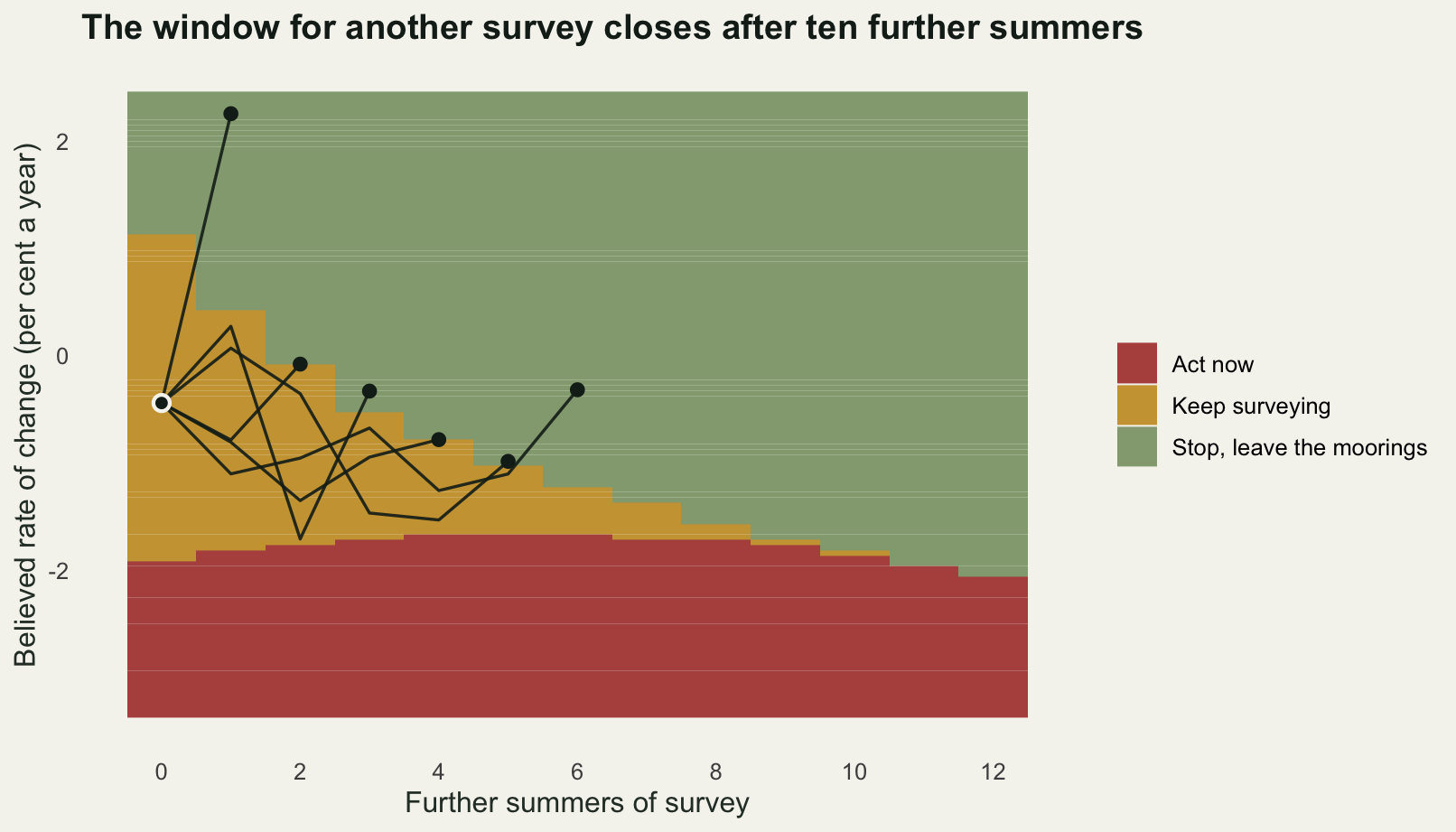
Two more summers, not ten
The rule can now be run forward against rules that people actually use. Every replicate draws a true rate from the current posterior, generates a true cover path, generates the August surveys along it, refits the slope each year, and hands the running slope to four policies. The optimal one stops when the belief leaves the window. The second stops at once and takes the terminal decision on the data in hand. The third surveys for ten more summers because ten is a round number and then takes the same terminal decision. The fourth surveys until the one-sided test for a decline gives a p-value below 0.05, acts at that point, and gives up if 25 further summers pass without significance. That fourth rule is given the true survey standard deviation rather than an estimate of it, which makes it stronger than its field version.
Costs are accumulated from the simulated cover path rather than from the formula the policies use, so the comparison does not run on the decision model’s own arithmetic.
cost_path <- function(xx, ks, act) {
  x_k <- xx[cbind(seq_len(nrow(xx)), ks + 1)]
  ks * c_surv + d_loss * pmax(0, -x_k) +
    ifelse(act, c_act, d_loss * pmax(0, -(xx[, horizon + 1] - x_k)))
}
pol_sig <- function(mm, alpha = 0.05) {
  ks <- rep(NA_integer_, nrow(mm))
  for (k in 0:k_max) {
    op <- is.na(ks); if (!any(op)) break
    ks[op & pnorm(mm[, k + 1] / (s_obs / sqrt(sxx(n_hist + k)))) < alpha] <- k
  }
  ks[is.na(ks)] <- k_max; ks
}
eval_pol <- function(s, ks, fa = NULL) {
  ms <- s$mm[cbind(seq_len(nrow(s$mm)), ks + 1)]
  act <- if (is.null(fa)) g_act_flag(ms, ks) else fa
  cc <- cost_path(s$xx, ks, act)
  c(cost = mean(cc), mc_se = sd(cc) / sqrt(length(cc)),
    mean_years = mean(ks), prob_acts = mean(act))
}

k_opt <- pol_opt(sm$mm)
k_sig <- pol_sig(sm$mm)
zero_k <- rep(0L, n_rep)
res <- rbind(optimal = eval_pol(sm, k_opt),
             stop_today = eval_pol(sm, zero_k),
             ten_more_summers = eval_pol(sm, rep(10L, n_rep)),
             wait_for_significance = eval_pol(sm, k_sig, fa = k_sig < k_max))
print(round(res, 3))
cost mc_se mean_years prob_acts
optimal 189.801 1.012 2.177 0.350
stop_today 241.719 1.823 0.000 0.000
ten_more_summers 284.205 1.258 10.000 0.255
wait_for_significance 326.830 0.617 15.825 0.524round(c(backward_induction_value = v_at(sol, m0, 0),
simulated_value = res[1, 1],
discrepancy_in_mc_standard_errors =
(res[1, 1] - v_at(sol, m0, 0)) / res[1, 2]), 4) backward_induction_value simulated_value
190.7868 189.8012
discrepancy_in_mc_standard_errors
-0.9744 print(table(k_opt))k_opt
1 2 3 4 5 6 7 8 9
11214 9288 5087 2642 1147 450 123 44 5 round(c(median_stop = median(k_opt), ninetieth_percentile = quantile(k_opt, 0.9),
longest_stop = max(k_opt),
never_significant = mean(k_sig == k_max),
excess_of_significance_rule = res[4, 1] - res[1, 1],
excess_as_share_of_works = (res[4, 1] - res[1, 1]) / c_act,
excess_of_ten_more = res[3, 1] - res[1, 1],
excess_of_stopping_today = res[2, 1] - res[1, 1],
ten_more_over_stopping_today = res[3, 1] - res[2, 1]), 4) median_stop ninetieth_percentile.90%
2.0000 4.0000
longest_stop never_significant
9.0000 0.4755
excess_of_significance_rule excess_as_share_of_works
137.0290 0.5270
excess_of_ten_more excess_of_stopping_today
94.4035 51.9175
ten_more_over_stopping_today
42.4860 The backward induction says the programme is worth 190.7868 thousand pounds of expected cost. The simulation, which shares no code with it, says 189.8012 with a Monte Carlo standard error of 1.012, a discrepancy of 0.9744 standard errors. The rule is what the recursion says it is.
Under that rule the median programme runs for two more summers, the ninetieth percentile is four, and the longest run in 30000 replicates is nine. Not one replicate reaches the tenth year, because the window has already closed by then. Stopping today instead costs 51.9175 thousand more. Surveying for ten more summers costs 94.4035 thousand more than the rule and 42.486 thousand more than doing no further monitoring at all, so the round number is worse than not monitoring.
Waiting for significance is the expensive one. It surveys for 15.825 further summers on average, fails to reach significance at all in 0.4755 of replicates, and costs 137.029 thousand more than the optimal rule, which is 0.5270 of the entire price of the works it is trying to authorise. The reason is visible in the decomposition below: the rule spends 142.43 thousand on diving against 19.59 for the optimal rule, and then acts more often than the economics warrant, because a significant slope is not the same event as a slope worth 260 thousand pounds.
decomp <- function(s, ks, fa = NULL) {
  ms <- s$mm[cbind(seq_len(nrow(s$mm)), ks + 1)]
  act <- if (is.null(fa)) g_act_flag(ms, ks) else fa
  x_k <- s$xx[cbind(seq_len(nrow(s$xx)), ks + 1)]
  c(Surveys = mean(ks * c_surv),
    `Loss while deciding` = mean(d_loss * pmax(0, -x_k)),
    `The works` = mean(ifelse(act, c_act, 0)),
    `Loss after leaving it` = mean(ifelse(act, 0,
                                    d_loss * pmax(0, -(s$xx[, horizon + 1] - x_k)))))
}
dc <- rbind(decomp(sm, k_opt), decomp(sm, zero_k), decomp(sm, rep(10L, n_rep)),
            decomp(sm, k_sig, fa = k_sig < k_max))
rule_lab <- c("Optimal rule\n(median 2 summers)", "Stop today\n(0 summers)",
              "Ten more summers", "Wait for p below 0.05\n(mean 15.8 summers)")
rownames(dc) <- rule_lab
print(round(dc, 2))
Surveys Loss while deciding
Optimal rule\n(median 2 summers) 19.59 17.94
Stop today\n(0 summers) 0.00 0.00
Ten more summers 90.00 80.57
Wait for p below 0.05\n(mean 15.8 summers) 142.43 47.29
The works Loss after leaving it
Optimal rule\n(median 2 summers) 90.97 61.30
Stop today\n(0 summers) 0.00 241.72
Ten more summers 66.35 47.28
Wait for p below 0.05\n(mean 15.8 summers) 136.36 0.75round(c(totals = rowSums(dc)), 3) totals.Optimal rule\n(median 2 summers)
189.801
totals.Stop today\n(0 summers)
241.719
totals.Ten more summers
284.205
totals.Wait for p below 0.05\n(mean 15.8 summers)
326.830 bars <- data.frame(rule = factor(rep(rule_lab, 4), levels = rule_lab),
part = factor(rep(colnames(dc), each = 4), levels = colnames(dc)),
value = as.vector(dc))
tot <- data.frame(rule = factor(rule_lab, levels = rule_lab), value = rowSums(dc))
ggplot(bars, aes(rule, value, fill = part)) +
geom_col(width = 0.62) +
geom_text(data = tot, aes(rule, value + 13, label = sprintf("%.0f", value)),
inherit.aes = FALSE, colour = te_pal$ink, size = 3.6, fontface = "bold") +
scale_fill_manual(values = c(Surveys = te_pal$gold,
`Loss while deciding` = te_pal$clay,
`The works` = te_pal$forest,
`Loss after leaving it` = te_pal$sage), name = NULL) +
scale_y_continuous(limits = c(0, 360)) +
labs(x = NULL, y = "Expected cost (GBP thousand)",
title = "Stopping after two summers beats every rule in common use") +
theme_te() +
theme(legend.position = "right")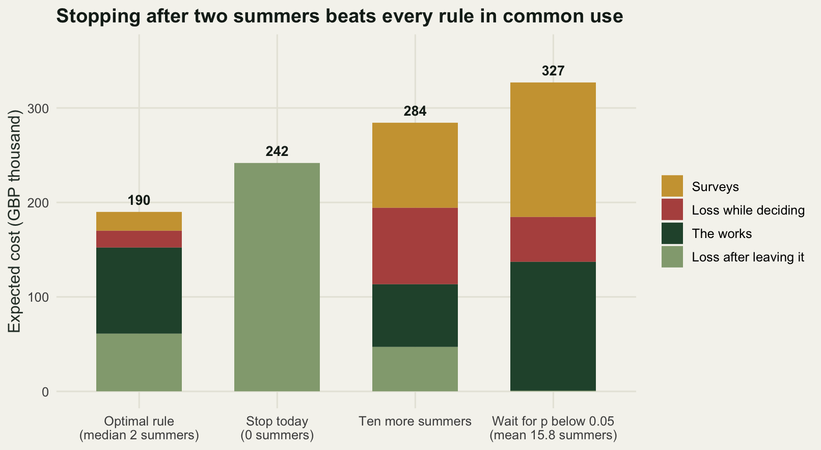
Power and decision relevance are different questions
The obvious objection is that two more summers cannot possibly be enough, because nobody could publish a trend on eleven points that noisy. That objection is correct about the statistics and beside the point about the decision, and the gap between the two is measurable.
pow_at <- function(n, b = beta_true, alpha = 0.05)
  pnorm(qnorm(alpha) - b / (s_obs / sqrt(sxx(n))))
n_80 <- (9:80)[which(sapply(9:80, pow_at) >= 0.8)[1]]
round(c(power_now = pow_at(n_hist),
        power_at_median_stop = pow_at(n_hist + median(k_opt)),
        mean_power_at_stopping = mean(pow_at(n_hist + k_opt)),
        summers_for_80_per_cent_power = n_80,
        power_there = pow_at(n_80),
        further_summers_needed = n_80 - n_hist), 4)
power_now power_at_median_stop
0.1486 0.2035
mean_power_at_stopping summers_for_80_per_cent_power
0.2127 24.0000
power_there further_summers_needed
0.8396 15.0000 At the year the rule stops, the power of a one-sided test to detect the decline that is actually happening averages 0.2127, and at the median stopping year it is 0.2035. To reach 80 per cent power on this design takes 24 summers, 15 more than are in hand, and by then the decision has been open for half the management horizon. The rule stops in a state that no monitoring report would describe as conclusive, and stopping there is still the cheapest thing to do, because the decision does not need the trend resolved. It needs to know which side of 260 thousand pounds the expected loss falls on, and that question is answered long before the slope is significant.
Where more data is worth less than the delay
The interesting failure of intuition is that the two things people mean by “we still do not know” come apart. There is decision relevant uncertainty, measured by what perfect knowledge of the trend would be worth, and there is the case for buying more of the data that is on offer. The first can be large while the second is zero.
evpi_k <- function(m, k, dl = d_loss) {
  v <- post_var(k); s <- sqrt(v); hh <- horizon - k
  rstar <- c_act / (dl * hh)
  za <- (-rstar - m) / s; zb <- -m / s
  tail_bit <- -(m * (pnorm(zb) - pnorm(za)) - s * (dnorm(zb) - dnorm(za)))
  pmin(c_act, hh * dl * er_mean(m, v)) - (c_act * pnorm(za) + dl * hh * tail_bit)
}
evpi_num <- function(m, k, dl = d_loss) {
  v <- post_var(k); hh <- horizon - k
  min(c_act, hh * dl * er_mean(m, v)) -
    integrate(function(b) pmin(c_act, hh * dl * pmax(0, -b)) * dnorm(b, m, sqrt(v)),
              -1, 1)$value
}
m_ev <- c(-0.03, cont_lo[1], m0, cont_hi[1])
print(round(rbind(belief = m_ev, closed_form = evpi_k(m_ev, 0),
                  numerical = sapply(m_ev, evpi_num, k = 0)), 5))
[,1] [,2] [,3] [,4]
belief -0.03000 -0.01900 -0.00441 0.01100
closed_form 40.46038 76.16695 122.33479 40.18323
numerical 40.46043 76.16701 122.33486 40.18326gain <- g_stop(m_grid, 0) - sol$value[[1]]
round(c(evpi_today = evpi_k(m0, 0),
value_of_monitoring_today = g_stop(m0, 0) - v_at(sol, m0, 0),
best_gain_anywhere = max(gain),
at_belief = m_grid[which.max(gain)]), 4) evpi_today value_of_monitoring_today best_gain_anywhere
122.3348 53.7042 60.7683
at_belief
-0.0055 round(c(lower_edge = cont_lo[1], per_cent_a_year = 100 * (exp(cont_lo[1]) - 1),
evpi_at_lower_edge = evpi_k(cont_lo[1], 0),
prob_not_declining_there = pnorm(0, cont_lo[1], sqrt(vk[1]),
lower.tail = FALSE),
evpi_at_upper_edge = evpi_k(cont_hi[1], 0),
prob_declining_there = pnorm(0, cont_hi[1], sqrt(vk[1]))), 4) lower_edge per_cent_a_year evpi_at_lower_edge
-0.0190 -1.8821 76.1669
prob_not_declining_there evpi_at_upper_edge prob_declining_there
0.2068 40.1832 0.3180 At the lower edge of the window, a believed decline of 1.88 per cent a year, the rule says stop surveying and commit the 260 thousand. At that same belief the probability that the meadow is not declining at all is 0.2068, and perfect knowledge of the trend would be worth 76.1669 thousand pounds against works costing 260. A fifth of the time the money is about to be spent on a meadow that is fine, resolving that would be worth a large fraction of the price of the works, and the correct action is still to stop looking. Perfect information is not on sale. What is on sale is one August of diving with a standard error of 0.18, and it does not arrive fast enough to be worth the year it takes.
The same point can be made by holding the belief fixed and moving the cost of delay, which changes nothing at all about how much is known.
mon_val <- function(dl) approx(m_grid, g_stop(m_grid, 0, dl) -
                                 solve_stop(dl = dl)$value[[1]], xout = m0)$y
dl_try <- c(200, 400, 600, 700, 1000, 1400, 1800, 2100, 2400)
print(round(rbind(delay_cost = dl_try, value_of_monitoring = sapply(dl_try, mon_val)), 3))
[,1] [,2] [,3] [,4] [,5] [,6] [,7]
delay_cost 200 400 600.000 700.000 1000.000 1400.000 1800.000
value_of_monitoring 0 0 31.389 53.711 43.606 22.843 8.566
[,8] [,9]
delay_cost 2100.000 2400
value_of_monitoring 0.349 0bisect <- function(lo_d, hi_d) {
for (it in 1:14) {
mid <- (lo_d + hi_d) / 2
if (mon_val(mid) > 1e-6) lo_d <- mid else hi_d <- mid
}
(lo_d + hi_d) / 2
}
upper_d <- bisect(1000, 3000)
lower_d <- bisect(1000, 150)
round(c(monitoring_pays_from = lower_d, monitoring_pays_to = upper_d,
evpi_at_upper = evpi_k(m0, 0, upper_d),
evpi_at_lower = evpi_k(m0, 0, lower_d),
posterior_sd_throughout = sqrt(vk[1])), 5) monitoring_pays_from monitoring_pays_to evpi_at_upper
406.98700 2174.62158 119.23943
evpi_at_lower posterior_sd_throughout
38.74549 0.02324 Monitoring pays only for delay costs between 406.987 and 2174.6216 thousand pounds per unit of annual rate. Below the lower figure there is nothing to buy, because at today’s belief the works are a long way from paying and a further August would only rarely move the belief far enough to change that, so the decision is settled. At the lower figure itself, resolving the trend completely would still be worth 38.74549 thousand pounds, while the monitoring on offer is worth nothing. Above the upper figure the expected value of perfect information is 119.23943 thousand pounds, the posterior standard deviation is the same 0.02324 it has been throughout, and the optimal number of further surveys is zero. More data would still be genuinely useful. It is simply worth less than what the meadow loses while the data is being collected. That is the sentence a monitoring programme rarely hears, and it is the whole content of a stopping rule.
sel <- m_grid >= -0.05 & m_grid <= 0.035
val_df <- data.frame(
  pct = rep(100 * (exp(m_grid[sel]) - 1), 2),
  value = c(evpi_k(m_grid[sel], 0), gain[sel]),
  what = factor(rep(c("Resolving the trend completely",
                      "The monitoring actually on offer"), each = sum(sel)),
                levels = c("Resolving the trend completely",
                           "The monitoring actually on offer")))

ggplot(val_df, aes(pct, value, colour = what)) +
  annotate("rect", xmin = 100 * (exp(cont_lo[1]) - 1),
           xmax = 100 * (exp(cont_hi[1]) - 1), ymin = 0, ymax = 130,
           fill = te_pal$gold, alpha = 0.18) +
  geom_line(linewidth = 1.05) +
  geom_vline(xintercept = 100 * (exp(m0) - 1), linetype = "dashed",
             colour = te_pal$ink, linewidth = 0.5) +
  annotate("text", x = 100 * (exp(m0) - 1) + 0.12, y = 126, hjust = 0, size = 3.1,
           colour = "#2c3a31", label = "today") +
  scale_colour_manual(values = c(te_pal$clay, te_pal$forest), name = NULL) +
  scale_y_continuous(limits = c(0, 132)) +
  labs(x = "Believed rate of change (per cent a year)",
       y = "Value of the information (GBP thousand)",
       title = "Most of what is worth knowing here is not worth buying") +
  theme_te() +
  theme(legend.position = "right")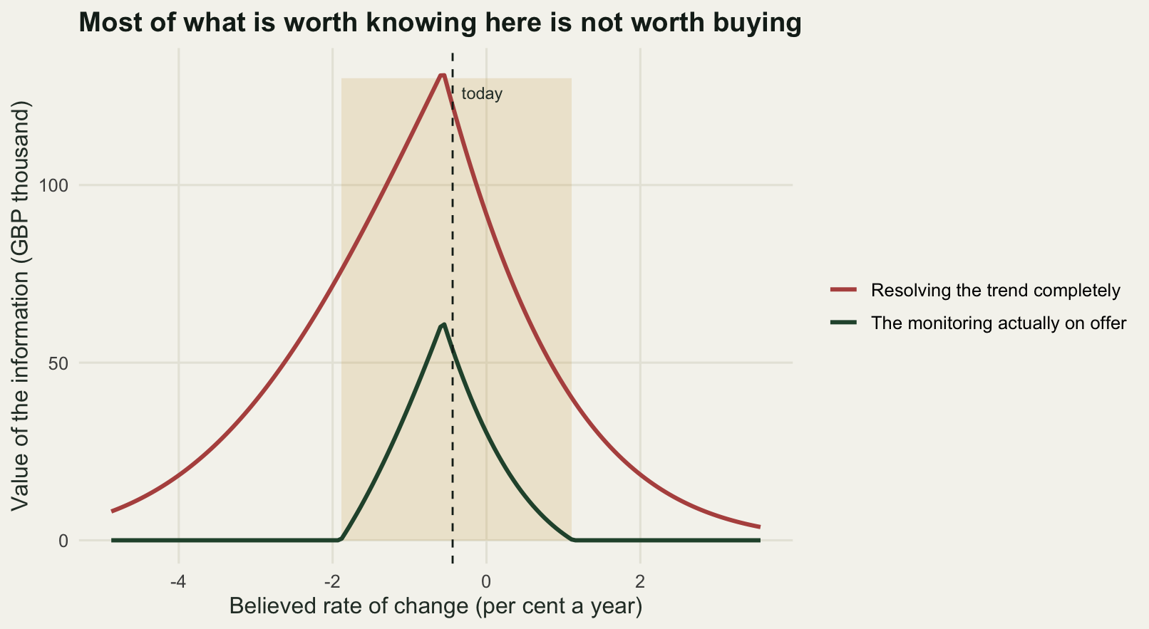
Which lever moves the stopping time
Two quantities in this problem are the ones a manager might actually be able to change or argue about: the cost of delay, which is a value judgement dressed as an exchange rate, and the survey standard deviation, which is a design choice about how many transects get dived. Sweeping both gives two measurements: how long monitoring could ever be worth doing, and how long it would actually run from today’s belief. The survey standard deviation is swept as a property of the whole programme, past and future, with the fitted rate held where it is, so the columns answer the question of what the answer would have been under a better or worse design all along.
sim_belief <- function(nrep, seed, so) {
  set.seed(seed)
  ssd <- sqrt(-diff(post_var(0:k_max, so)))
  mm <- matrix(0, nrep, k_max + 1); mm[, 1] <- m0
  for (k in 1:k_max) mm[, k + 1] <- mm[, k] + ssd[k] * rnorm(nrep)
  mm
}
cell <- function(dl, so, nrep = 4000) {
  s <- solve_stop(dl = dl, so = so)
  loc <- sapply(s$continue, function(z) if (any(z)) min(m_grid[z]) else NA)
  hic <- sapply(s$continue, function(z) if (any(z)) max(m_grid[z]) else NA)
  ks <- pol_opt(sim_belief(nrep, 20260723, so), loc, hic)
  anyc <- sapply(s$continue, any)
  c(years = mean(ks), hor = if (any(anyc)) max(which(anyc)) - 1 else 0)
}
dl_v <- c(200, 300, 450, 700, 1000, 1500, 2200)
so_v <- c(0.09, 0.12, 0.15, 0.18, 0.22, 0.27, 0.33)
grid_sw <- expand.grid(delay_cost = dl_v, survey_sd = so_v)
out_sw <- t(mapply(cell, grid_sw$delay_cost, grid_sw$survey_sd))
hor_m <- matrix(out_sw[, "hor"], length(dl_v), dimnames = list(dl_v, so_v))
yrs_m <- matrix(out_sw[, "years"], length(dl_v), dimnames = list(dl_v, so_v))
print(hor_m)
0.09 0.12 0.15 0.18 0.22 0.27 0.33
200 0 1 2 3 4 5 6
300 1 3 4 5 6 7 8
450 3 5 6 7 8 9 10
700 6 7 8 10 11 12 13
1000 7 9 10 11 12 14 15
1500 10 11 13 13 15 16 17
2200 12 13 14 15 17 18 19print(round(yrs_m, 2)) 0.09 0.12 0.15 0.18 0.22 0.27 0.33
200 0.00 0.00 0.00 0.00 0.00 0.00 0.00
300 0.00 0.00 0.00 0.00 0.00 1.51 1.80
450 0.00 0.00 0.00 1.57 1.85 2.14 2.38
700 0.00 1.71 1.98 2.20 2.39 2.54 2.59
1000 1.84 2.18 2.37 2.48 2.50 2.57 2.50
1500 2.21 2.36 2.40 2.40 2.42 2.36 0.00
2200 2.23 2.27 2.26 0.00 0.00 0.00 0.00round(c(horizon_span_along_delay_cost = mean(apply(hor_m, 2, function(z) diff(range(z)))),
horizon_span_along_survey_sd = mean(apply(hor_m, 1, function(z) diff(range(z)))),
cells_with_no_monitoring = sum(yrs_m == 0),
cells_with_monitoring = sum(yrs_m > 0), cells_total = length(yrs_m),
shortest_positive_run = min(yrs_m[yrs_m > 0]),
longest_run = max(yrs_m)), 4)horizon_span_along_delay_cost horizon_span_along_survey_sd
12.4286 7.0000
cells_with_no_monitoring cells_with_monitoring
21.0000 28.0000
cells_total shortest_positive_run
49.0000 1.5085
longest_run
2.5867 The two measurements disagree, and the disagreement is the finding. The monitoring horizon, the last year at which another survey could ever be justified for some belief, is driven mainly by the cost of delay: moving that cost across the swept range shifts the horizon by 12.4286 years on average, while moving the survey standard deviation from 0.09 to 0.33 shifts it by 7. Expensive delay buys a long option; when delay is cheap the decision is not worth resolving and the option closes early. Nothing surprising there.
The number of summers actually surveyed behaves differently. In 21 of the 49 combinations it is exactly zero, because the decision is already settled at today’s belief, either because the meadow is clearly not worth the works or because it clearly is. In the other 28 it lies between 1.5085 and 2.5867. There is no dial here. Across the whole sweep of delay cost and survey precision, a live decision of this shape takes about two more summers, or none, and the parameters mostly decide which of those two it is rather than how many years.
sw_df <- rbind(
  data.frame(grid_sw, value = out_sw[, "hor"], lab = sprintf("%d", out_sw[, "hor"]),
             panel = "Last year another survey could pay"),
  data.frame(grid_sw, value = out_sw[, "years"], lab = sprintf("%.1f", out_sw[, "years"]),
             panel = "Summers actually surveyed from today"))
sw_df$panel <- factor(sw_df$panel, levels = unique(sw_df$panel))
sw_df$scaled <- ave(sw_df$value, sw_df$panel, FUN = function(z) z / max(z))

ggplot(sw_df, aes(factor(survey_sd), factor(delay_cost), fill = scaled)) +
  geom_tile(colour = te_pal$paper, linewidth = 1) +
  geom_text(aes(label = lab, colour = scaled > 0.55), size = 3.2, show.legend = FALSE) +
  facet_wrap(~panel) +
  scale_fill_gradient(low = "#e8e6d8", high = te_pal$forest, guide = "none") +
  scale_colour_manual(values = c("TRUE" = te_pal$paper, "FALSE" = te_pal$ink)) +
  labs(x = "Survey standard deviation on the log scale",
       y = "Loss per unit annual rate (GBP thousand)",
       title = "The cost of delay sets the option; it barely sets the answer") +
  theme_te() +
  theme(panel.grid.major = element_blank(),
        strip.text = element_text(colour = te_pal$ink, face = "bold"))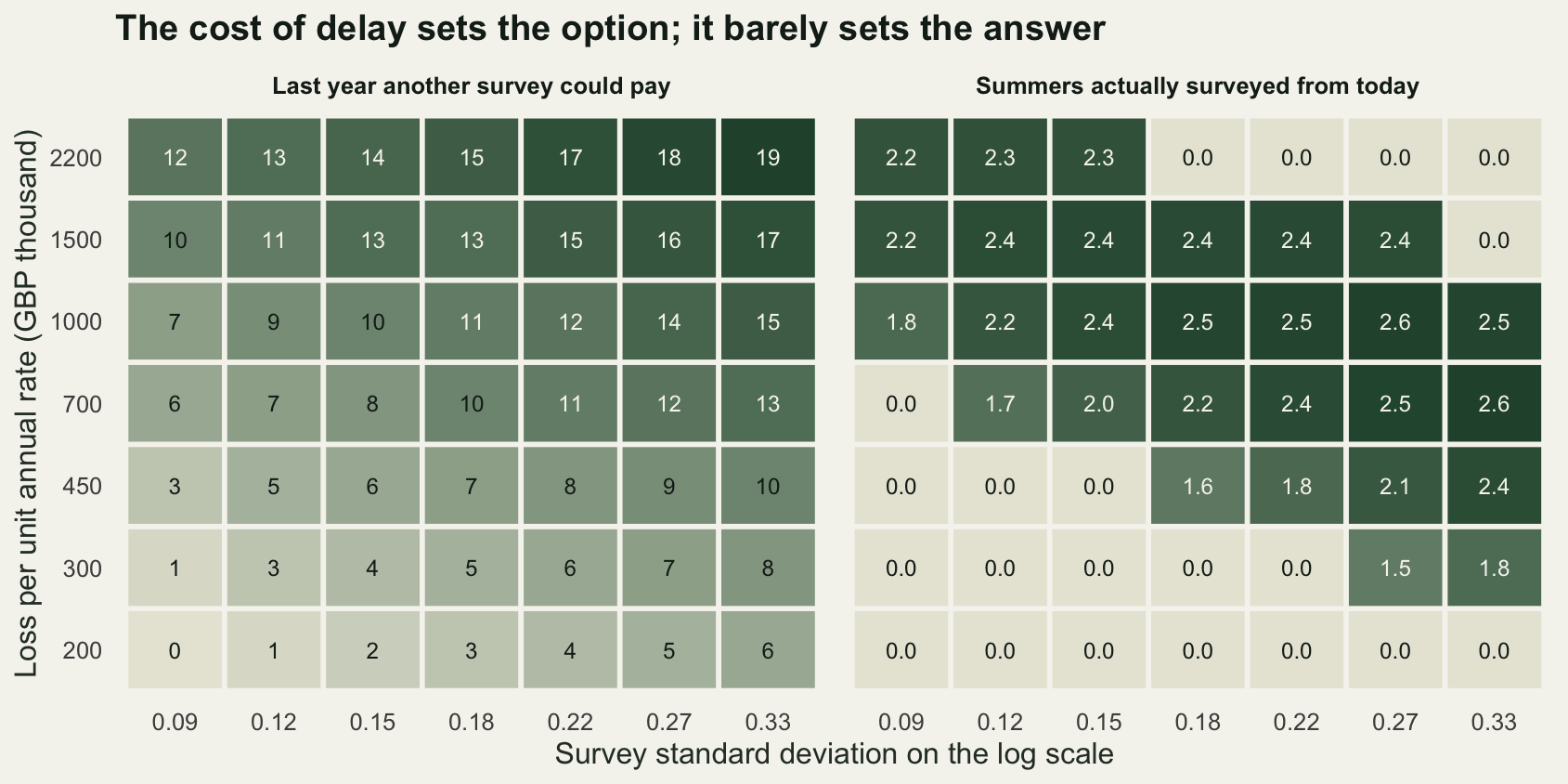
The honest limit
The rule above assumes the meadow has one rate of change and keeps it for 30 years. Seagrass does not behave like that. Beds sit still for a decade and then go in three years when a threshold in light or sediment is crossed, and a stopping rule fitted to a straight line will stop before any of that is visible. The cheapest way to find out how much that matters is to keep the rule exactly as derived and generate the truth from a trend that wanders.
drift_run <- function(ps) {
  s2 <- sim_fwd(n_rep, 20260723, proc_sd = ps)
  ko <- pol_opt(s2$mm); kg <- pol_sig(s2$mm)
  c(optimal = eval_pol(s2, ko)["cost"],
    stop_today = eval_pol(s2, rep(0L, n_rep))["cost"],
    ten_more = eval_pol(s2, rep(10L, n_rep))["cost"],
    significance = eval_pol(s2, kg, fa = kg < k_max)["cost"],
    years = eval_pol(s2, ko)["mean_years"])
}
drift <- t(sapply(c(0, 0.004, 0.008), drift_run))
rownames(drift) <- c("no drift", "drift sd 0.004", "drift sd 0.008")
print(round(drift, 2))
optimal.cost stop_today.cost ten_more.cost significance.cost
no drift 189.80 241.72 284.20 326.83
drift sd 0.004 210.22 269.66 309.66 337.82
drift sd 0.008 256.46 337.27 360.28 358.09
years.mean_years
no drift 2.18
drift sd 0.004 2.17
drift sd 0.008 2.17round(c(penalty_at_0.004 = drift[2, 1] - drift[1, 1],
penalty_at_0.008 = drift[3, 1] - drift[1, 1],
margin_over_stopping_today_no_drift = drift[1, 2] - drift[1, 1],
margin_over_stopping_today_at_0.008 = drift[3, 2] - drift[3, 1]), 3) penalty_at_0.004 penalty_at_0.008
20.420 66.657
margin_over_stopping_today_no_drift margin_over_stopping_today_at_0.008
51.917 80.809 Letting the annual rate wander with a standard deviation of 0.004 a year costs the rule 20.42 thousand pounds of expected value, and doubling that to 0.008 costs 66.657. The rule is misspecified and it pays for it. What does not happen is a reversal: the margin over stopping today is 51.917 thousand with no drift and 80.809 thousand at the larger drift, so a wandering trend makes monitoring more valuable rather than less, and the rule stays first at every drift tried. The two naive rules do change places at the largest drift, where waiting for significance turns out marginally cheaper than ten fixed summers, which is a warning about how little either of them is tracking. A rule fitted to the wrong dynamics is still better here than no rule, and that is the most that can be claimed for it.
Three other limits do not have numbers attached, and should not be given any. The exchange rate of 700 thousand pounds per unit of annual decline rate is a value judgement, and every threshold above moves with it, which is why the sweep was run at all; the machinery for eliciting a number like that lives in structured decision making in R and it does not come out of any survey. The assumption that the works halt the decline outright is generous, and a partially effective intervention shifts the action threshold upwards. And the whole calculation prices monitoring for one decision only. The same August dive detects the arrival of an invasive alga, keeps a designated feature under formal surveillance, and holds a mooring association to an agreement, and none of those appear anywhere in the cost function. A stopping rule for one decision is not a case for closing a monitoring programme. It is an answer to the question of how long that one decision should be allowed to wait, which was the question asked in November.
Where to go next
The natural next step is to let the action be more than a switch. Here the manager either replaces the moorings or does not, and the meadow’s state enters only through the belief about its trend. When the state itself is the thing being managed, and today’s action changes what is available next year, the machinery becomes a Markov decision process, and markov decision processes for management builds one from an explicit transition model. The other direction is design rather than duration: revisit designs for monitoring asks how the same survey effort should be spread over sites and years, which changes the rate at which the posterior variance falls and therefore changes every threshold computed above.
References
Wald A 1947 Sequential Analysis. Wiley; Dover reprint 1973, ISBN 978-0-486-61579-0
Bellman R 2010 Dynamic Programming. Princeton University Press, ISBN 978-0-691-14668-3
DeGroot MH 2004 Optimal Statistical Decisions. Wiley Classics Library, ISBN 978-0-471-68029-1
Legg CJ, Nagy L 2006 Journal of Environmental Management 78(2):194-199 (10.1016/j.jenvman.2005.04.016)
Gerrodette T 1987 Ecology 68(5):1364-1372 (10.2307/1939220)