library(ggplot2)

te_pal <- list(forest = "#275139", green = "#2f8f63", sage = "#93a87f",
               clay = "#b5534e", gold = "#cda23f", line = "#dad9ca",
               ink = "#16241d", paper = "#f5f4ee")

theme_te <- function() {
  theme_minimal(base_size = 12) +
    theme(panel.grid.minor = element_blank(),
          panel.grid.major = element_line(colour = "#e7e6dc"),
          plot.background = element_rect(fill = "#f5f4ee", colour = NA),
          panel.background = element_rect(fill = "#f5f4ee", colour = NA),
          plot.title = element_text(face = "bold", colour = te_pal$ink),
          axis.title = element_text(colour = "#2c3a31"),
          axis.text = element_text(colour = "#2c3a31"))
}Testing a monitoring series every year
R
monitoring
multiple testing
trend
ecology tutorial
Retesting a monitoring trend every year inflates the false alarm rate more than sixfold. Simulation in R prices the damage and two boundaries that fix it.
A chalk grassland reserve counts flowering spikes of a scarce orchid on thirty permanent plots, once a year, in the same fortnight of June, by the same protocol. The count has run for twenty-five years. Every autumn the warden adds the new year to the spreadsheet, fits a line through the log of the annual mean, and looks at whether the slope differs from zero. The question is always the same question: is this population going down?
Nothing about that sounds like a statistical error. The data are as good as monitoring data get, the model is the standard one, the test is two-sided at five per cent, and the warden is not fishing for a result. The only unusual thing is the repetition. The same null hypothesis, about the same population, is tested twenty-one times over twenty-one years, and each test uses all the data that went into the previous one plus one new point.
That repetition has a price, and the price is not small. A test with a five per cent false alarm rate has that rate once. Run it every year on a growing series and the probability that it fires at least once is a different number entirely, and the year it fires is not random either: it tends to fire early, when the series is short, the slope estimate is at its noisiest, and the estimate that comes with the alarm is at its most extreme. A programme that stops and reports at that moment publishes a decline steeper than the one it was looking for.
This post measures all of that on simulated counts with the true trend known, then prices two standard repairs. It sits next to three posts and repeats none of them. When to stop monitoring prices a further year of survey by backward induction, and one of its results is what waiting for a significant slope costs in decision terms; it never measures the false alarm rate of that waiting rule, which is the first quantity below. Power to detect a population trend is fixed-horizon power: one test, at a horizon chosen in advance. Here the same test is run many times as the horizon grows, and the fixed-horizon calculation is the baseline that the annual habit departs from. Checking a multiple-testing analysis and the false discovery rate posts correct across different hypotheses tested at one time: many taxa, many sites, one screen. This is the other axis. One hypothesis, many times, with the tests strongly and unavoidably dependent, because year twelve’s data set contains the whole of year eleven’s. That dependence is why a Bonferroni correction across looks is the wrong tool, and it is also the structure that the sequential boundaries exploit.
The counts, the model and the annual test
Each plot has its own mean abundance, drawn on the log scale so that some plots are richer than others and stay that way. Every year carries a weather effect shared across the whole reserve, which is what makes annual index values wobble together. Each plot-year has its own departure on top of that, and the count itself is Poisson around the resulting expectation. The population trend is a constant on the log scale, so a trend of zero means the expected count in year twenty-five equals the expected count in year one.
The annual index is the log of the mean count per plot. Collapsing thirty plots to one figure a year before fitting the trend is the standard move for a fixed-plot scheme and it is the honest one: the weather effect is common to all plots, so treating plot-years as independent replicates would put the error term at the wrong scale. The trend model is then a linear model of the annual index on the year number, and the test is the two-sided t test on its slope.
n_plot <- 30
n_year <- 25
k_min <- 5
lam0 <- 40
sd_plot <- 0.40
sd_yr <- 0.15
sd_pt <- 0.35
alpha_nom <- 0.05
looks <- k_min:n_year
n_look <- length(looks)

sim_index <- function(slope_true) {
  a_i <- rnorm(n_plot, log(lam0), sd_plot)
  u_j <- rnorm(n_year, 0, sd_yr)
  e_ij <- matrix(rnorm(n_plot * n_year, 0, sd_pt), n_plot, n_year)
  eta <- outer(a_i, rep(1, n_year)) +
    outer(rep(1, n_plot), slope_true * (seq_len(n_year) - 1) + u_j) + e_ij
  log(colMeans(matrix(rpois(n_plot * n_year, exp(eta)), n_plot, n_year)))
}

print(c(plots = n_plot, years = n_year, first_look = k_min,
        number_of_looks = n_look, median_count_per_plot = lam0))
plots years first_look
30 25 5
number_of_looks median_count_per_plot
21 40 print(round(c(plot_sd = sd_plot, year_sd = sd_yr, plot_year_sd = sd_pt), 3)) plot_sd year_sd plot_year_sd
0.40 0.15 0.35 Refitting a linear model twenty-one times per simulated programme, several thousand times over, is wasteful when the fit has a closed form. The slope, its standard error and the t statistic at every look can be read off three cumulative sums, which is what the next function does. It returns one value per series length, from two years up to the full twenty-five, and the looks actually used start at 5 years, which is the shortest series anybody would put a trend line through.
look_stats <- function(y) {
  kk <- seq_along(y)
  s1 <- cumsum(y)
  sxy <- cumsum(kk * y)
  sy2 <- cumsum(y^2)
  sx <- cumsum(kk)
  sx2 <- cumsum(kk^2)
  Sxx <- sx2 - sx^2 / kk
  Sxy <- sxy - sx * s1 / kk
  Syy <- sy2 - s1^2 / kk
  sl <- Sxy / Sxx
  se <- sqrt(pmax(Syy - Sxy^2 / Sxx, 0) / ((kk - 2) * Sxx))
  list(slope = sl, se = se, tv = sl / se)
}

set.seed(20260801)
chk_y <- sim_index(0)
chk_st <- look_stats(chk_y)
chk_lm <- lm(chk_y ~ I(seq_len(n_year)))
rep_stat <- replicate(200, {
  y_r <- sim_index(0)
  st_r <- look_stats(y_r)
  c(idx_sd = sd(y_r), se_5 = st_r$se[k_min], se_25 = st_r$se[n_year])
})
idx_sd <- mean(rep_stat["idx_sd", ])
se_5 <- mean(rep_stat["se_5", ])
se_25 <- mean(rep_stat["se_25", ])

print(round(c(closed_form_slope = chk_st$slope[n_year],
              lm_slope = unname(coef(chk_lm)[2]),
              closed_form_se = chk_st$se[n_year],
              lm_se = summary(chk_lm)$coefficients[2, 2]), 8))
closed_form_slope lm_slope closed_form_se lm_se
0.00557098 0.00557098 0.00498949 0.00498949 print(round(c(index_sd_about_the_line = idx_sd,
mean_se_of_slope_at_25_years = se_25,
mean_se_of_slope_at_5_years = se_5,
se_ratio = se_5 / se_25), 5)) index_sd_about_the_line mean_se_of_slope_at_25_years
0.16638 0.00460
mean_se_of_slope_at_5_years se_ratio
0.05073 11.02066 The closed form agrees with lm to eight decimal places, so the shortcut is exact rather than approximate. The annual index scatters about its own trend line with a standard deviation of 0.1664 on the log scale, which is a fairly quiet monitoring series. At twenty-five years the standard error of the slope averages 0.0046 per year, so the smallest trend the full series can call significant is about 0.96 per cent a year. At five years the standard error averages 0.0507, a factor of 11 larger, which is the fact behind every early estimate below.
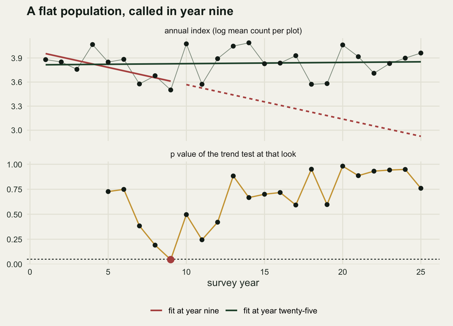
One programme, with the population held exactly flat, shows the shape of the problem.
set.seed(20261056)
ex_y <- sim_index(0)
ex_st <- look_stats(ex_y)
ex_p <- 2 * pt(-abs(ex_st$tv[looks]), looks - 2)
ex_first <- looks[which(ex_p < alpha_nom)[1]]

print(round(data.frame(year = looks, index = ex_y[looks],
                       trend = ex_st$slope[looks], p = ex_p)[1:9, ], 4))
year index trend p
1 5 3.8487 0.0156 0.7269
2 6 3.8829 0.0092 0.7487
3 7 3.5761 -0.0269 0.3833
4 8 3.6788 -0.0312 0.1910
5 9 3.5015 -0.0429 0.0461
6 10 4.0758 -0.0152 0.4965
7 11 3.5723 -0.0223 0.2445
8 12 3.8911 -0.0133 0.4204
9 13 4.0471 -0.0022 0.8830print(round(c(first_significant_year = ex_first,
trend_there = ex_st$slope[ex_first],
pct_per_year_there = 100 * (exp(ex_st$slope[ex_first]) - 1),
p_there = ex_p[looks == ex_first],
trend_at_25 = ex_st$slope[n_year],
p_at_25 = ex_p[n_look]), 4))first_significant_year trend_there pct_per_year_there
9.0000 -0.0429 -4.1996
p_there trend_at_25 p_at_25
0.0461 0.0015 0.7598 In year 9 this programme would have reported a decline of 4.2 per cent a year, p equal to 0.0461, from a population that was not moving. Sixteen years later the same series gives a trend of 0.0015 per year and a p value of 0.76. Nothing was done wrong at year 9. The model was right, the data were real, the test was the correct test.
The rate the programme actually runs at
One programme proves nothing, so the study runs several thousand of them under a true trend of exactly zero. Each replicate redraws the plot effects, the weather, the plot-year departures and the Poisson counts, computes the trend test at every look from year 5 to year 25, and stores the p value, the slope and its standard error at each.
run_study <- function(slope_true, seed, n_rep) {
  set.seed(seed)
  p_mat <- s_mat <- e_mat <- matrix(NA_real_, n_rep, n_look)
  for (b in seq_len(n_rep)) {
    st <- look_stats(sim_index(slope_true))
    p_mat[b, ] <- 2 * pt(-abs(st$tv[looks]), looks - 2)
    s_mat[b, ] <- st$slope[looks]
    e_mat[b, ] <- st$se[looks]
  }
  list(p = p_mat, slope = s_mat, se = e_mat)
}

n_rep <- 20000
nul <- run_study(0, 20260802, n_rep)

fixed_t1 <- mean(nul$p[, n_look] < alpha_nom)
any_hit <- rowSums(nul$p < alpha_nom) > 0
seq_t1 <- mean(any_hit)
mc_fixed <- sqrt(fixed_t1 * (1 - fixed_t1) / n_rep)
mc_seq <- sqrt(seq_t1 * (1 - seq_t1) / n_rep)

print(round(c(replicates = n_rep, looks_per_replicate = n_look), 0))
replicates looks_per_replicate
20000 21 print(round(c(fixed_horizon_type1 = fixed_t1, mc_se = mc_fixed), 5))fixed_horizon_type1 mc_se
0.05310 0.00159 print(round(c(annual_testing_type1 = seq_t1, mc_se = mc_seq,
inflation_factor = seq_t1 / fixed_t1), 4))annual_testing_type1 mc_se inflation_factor
0.3430 0.0034 6.4595 Over 20000 simulated programmes, tested once at year 25, the trend test has a false alarm rate of 0.0531 against a nominal 0.05, with a Monte Carlo standard error of 0.00159. That is the calibration check, and it passes: the fixed-horizon test does what it says.
Tested every year from year 5, the probability that the programme declares a significant trend at some point during its twenty-five years is 0.343, Monte Carlo standard error 0.00336. The inflation is a factor of 6.46. Roughly one flat population in three gets called, and the result of the call is a published trend with a p value below five per cent attached to it.
That number is a property of the habit, not of the data. Nobody has to p-hack, run a bad model or choose a convenient subset to get it. Armitage, McPherson and Rowe (1969) computed this inflation for the normal, binomial and exponential cases and it is the founding result of sequential testing; Simmons, Nelson and Simonsohn (2011) made the same point about optional stopping in experimental work, where collecting until significance is a decision about sample size rather than about years.
first_ix <- max.col(nul$p < alpha_nom, "first")
first_year <- looks[first_ix]
cum_hit <- function(cross) {
  ix <- max.col(cross, "first")
  hit <- rowSums(cross) > 0
  vapply(seq_len(n_look), function(j) mean(hit & ix <= j), numeric(1))
}
cum_naive <- cum_hit(nul$p < alpha_nom)
print(round(rbind(year = looks, cumulative_rate = cum_naive)[, c(1, 3, 6, 11, 16, 21)], 4))
[,1] [,2] [,3] [,4] [,5] [,6]
year 5.0000 7.0000 10.0000 15.000 20.0000 25.000
cumulative_rate 0.0498 0.1076 0.1734 0.247 0.3003 0.343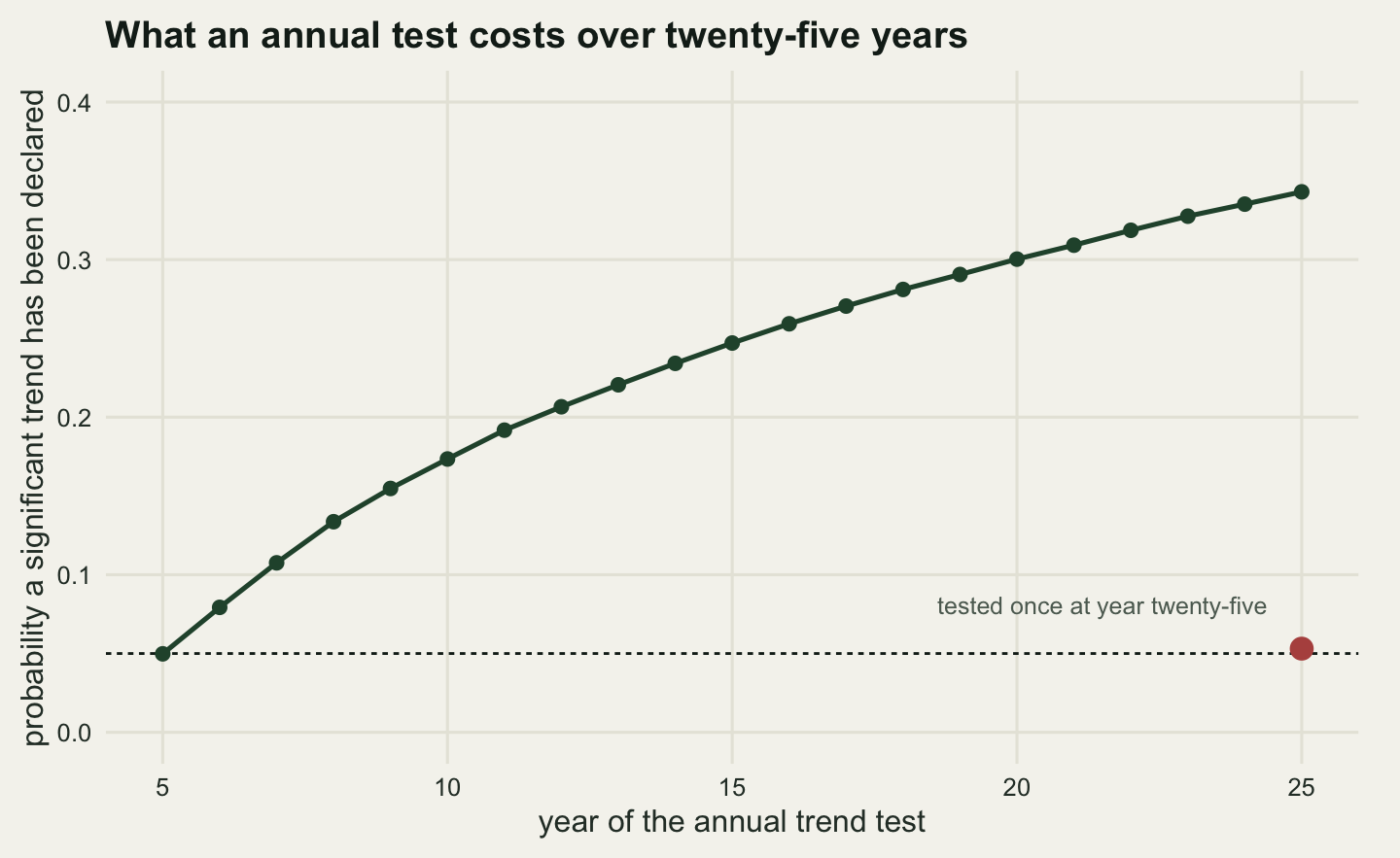
The false alarm arrives early
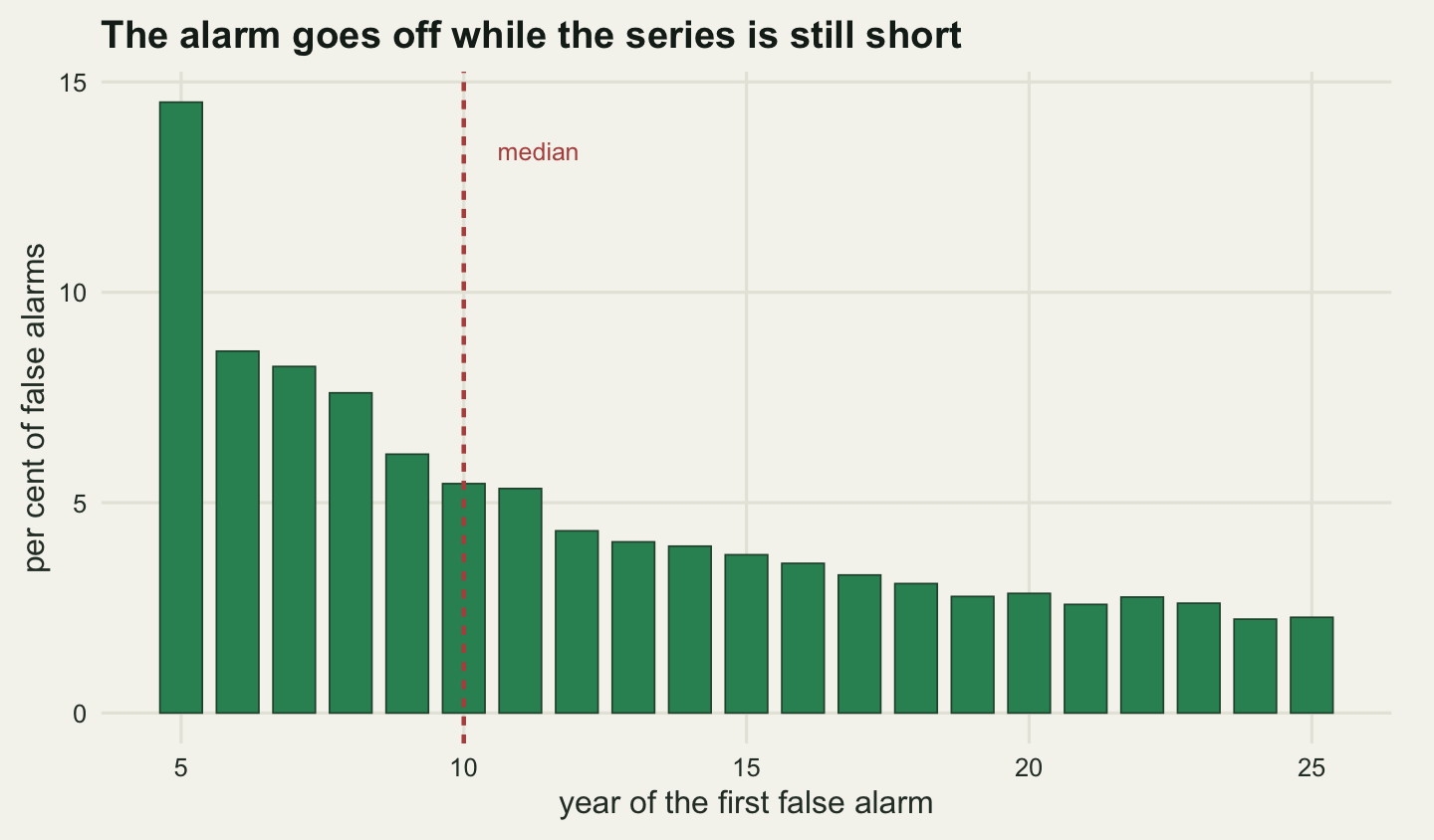
Where in the twenty-five years the alarm lands matters more than it looks. A false alarm in year twenty-two is embarrassing; a false alarm in year eight sets the direction of a programme that then runs for another seventeen years on the assumption that it found something.
alarm_year <- first_year[any_hit]
alarm_q <- quantile(alarm_year, c(0.25, 0.5, 0.75))
med_alarm <- unname(alarm_q[2])
lo_alarm <- unname(alarm_q[1])
hi_alarm <- unname(alarm_q[3])
print(round(c(n_alarms = length(alarm_year),
              median_year = med_alarm,
              lower_quartile = lo_alarm,
              upper_quartile = hi_alarm,
              share_by_year_10 = mean(alarm_year <= 10),
              share_by_year_12 = mean(alarm_year <= 12)), 4))
n_alarms median_year lower_quartile upper_quartile
6860.0000 10.0000 7.0000 16.0000
share_by_year_10 share_by_year_12
0.5057 0.6023 print(round(c(share_at_the_first_look = mean(alarm_year == k_min),
mean_se_at_first_look = se_5,
mean_se_at_last_look = se_25,
se_ratio = se_5 / se_25), 4))share_at_the_first_look mean_se_at_first_look mean_se_at_last_look
0.1452 0.0507 0.0046
se_ratio
11.0207 The median year of the first false alarm is 10, with quartiles at 7 and 16. Half of all false alarms have happened by year 10, and 14.52 per cent of them happen at the very first look, in year 5, which is the single most common year for a programme to fool itself.
Every look is a valid test at the nominal level on its own, and only the first has nothing in front of it: the later ones lose a growing share of theirs to the programmes that alarmed earlier. What the standard error sets is not the timing but the size of the estimate that comes with the call. At five years that error averages 0.0507 per year and at twenty-five years 0.0046, a ratio of 11.02, because the information in a trend test grows with the cube of the series length rather than with its length. An early look is a lottery with a large prize, and the annual habit buys a ticket every year, starting with the years where the prize is most misleading.
Why a Bonferroni correction across looks is the wrong tool
The instinct of anyone who has met multiple testing is to divide. Twenty-one looks, so test each at five per cent divided by twenty-one. That controls the overall rate, and it overcontrols it, because Bonferroni is built for the worst case in which the tests carry no shared information and this family is about as far from that case as a family gets.
cor_mat <- cor(nul$slope)
adj_cor <- mean(cor_mat[cbind(1:(n_look - 1), 2:n_look)])
a_bonf <- alpha_nom / n_look
bonf_t1 <- mean(rowSums(nul$p < a_bonf) > 0)
eff_looks <- log(1 - seq_t1) / log(1 - 0.05)

print(round(c(cor_look_5_and_6 = cor_mat[1, 2],
              cor_look_24_and_25 = cor_mat[n_look - 1, n_look],
              cor_look_15_and_25 = cor_mat[looks == 15, n_look],
              cor_look_5_and_25 = cor_mat[1, n_look],
              mean_adjacent_cor = adj_cor), 4))
cor_look_5_and_6 cor_look_24_and_25 cor_look_15_and_25 cor_look_5_and_25
0.7589 0.9397 0.4632 0.0853
mean_adjacent_cor
0.8875 print(round(c(bonferroni_per_look = a_bonf,
bonferroni_overall = bonf_t1,
budget_used = bonf_t1 / alpha_nom,
effective_independent_looks = eff_looks,
actual_looks = n_look), 4)) bonferroni_per_look bonferroni_overall
0.0024 0.0271
budget_used effective_independent_looks
0.5410 8.1896
actual_looks
21.0000 Successive slope estimates from the same growing series correlate at 0.887 on average, and the last two looks at 0.9397: adding a twenty-fifth point to a twenty-four point series barely moves the line. Distant looks are much less alike, 0.0853 between year 5 and year 25, because the early estimate is built from data that carry almost none of the final estimate’s information. So the family is neither independent nor redundant, and its effective size is somewhere in between: solving Sidak’s formula against the measured overall rate gives 8.19 independent looks in place of 21.
Bonferroni does not know that. Splitting five per cent across 21 looks gives a per-look level of 0.00238 and an overall false alarm rate of 0.0271, which is 54.1 per cent of the budget it was allowed to spend. The unspent half is power thrown away, and the section below puts a number on it. What the sequential boundaries of Pocock (1977) and O’Brien and Fleming (1979) do differently is take the joint distribution of the whole sequence of statistics into account rather than treating each look as a separate hypothesis, which is exactly what the positive dependence between looks makes possible.
The estimate that comes with the alarm
The false alarm rate is the familiar part of this problem. The part that catches people is what the stopped estimate looks like. Stopping at the first significant look is a selection rule, and it selects for extreme estimates, because an estimate has to be extreme to be significant on a short series.
alt_slope <- -0.015
alt <- run_study(alt_slope, 20260803, n_rep)

stopped_at <- function(run, cross, what) {
  ix <- max.col(cross, "first")
  hit <- rowSums(cross) > 0
  run[[what]][cbind(seq_len(n_rep), ix)][hit]
}
null_stop <- stopped_at(nul, nul$p < alpha_nom, "slope")
alt_hit <- rowSums(alt$p < alpha_nom) > 0
alt_stop <- stopped_at(alt, alt$p < alpha_nom, "slope")

print(round(c(truth = 0,
              mean_abs_slope_at_stopping = mean(abs(null_stop)),
              mean_abs_slope_at_year_25 = mean(abs(nul$slope[, n_look])),
              ratio = mean(abs(null_stop)) / mean(abs(nul$slope[, n_look])),
              pct_per_year_reported = 100 * (exp(mean(abs(null_stop))) - 1)), 4))
truth mean_abs_slope_at_stopping
0.0000 0.0425
mean_abs_slope_at_year_25 ratio
0.0037 11.3663
pct_per_year_reported
4.3461 print(round(c(truth = alt_slope,
mean_slope_at_stopping = mean(alt_stop),
mean_slope_at_year_25 = mean(alt$slope[, n_look]),
inflation_factor = mean(alt_stop) / alt_slope,
fixed_horizon_factor = mean(alt$slope[, n_look]) / alt_slope,
power_of_annual_testing = mean(alt_hit)), 4)) truth mean_slope_at_stopping mean_slope_at_year_25
-0.0150 -0.0262 -0.0150
inflation_factor fixed_horizon_factor power_of_annual_testing
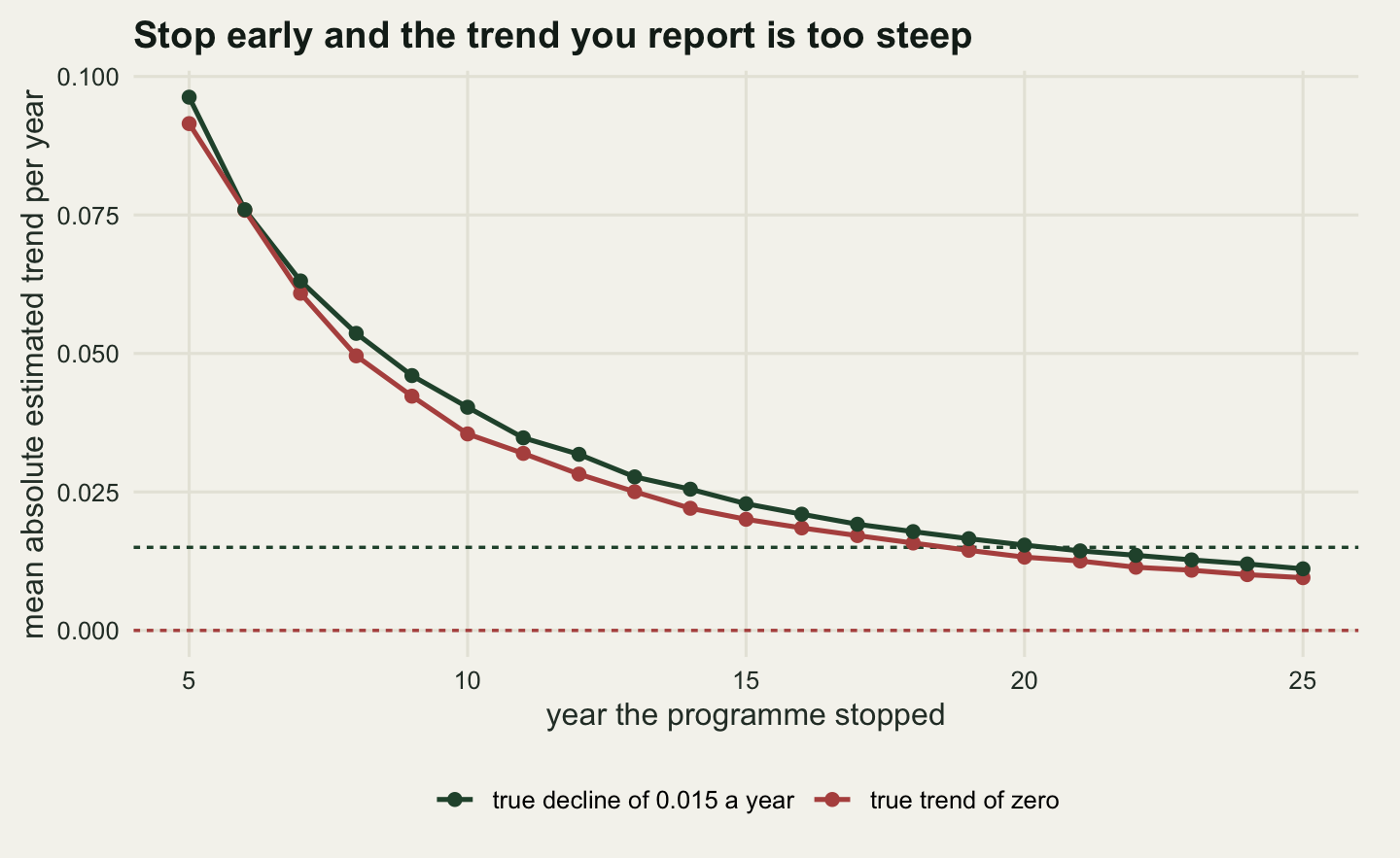
1.7480 0.9980 0.9295 Under a true trend of zero, the programmes that stopped report a mean absolute trend of 0.0425 per year, which is 4.35 per cent a year, against 0.0037 for the same estimator at the fixed horizon: a factor of 11.4. The truth is zero, so all of that is artefact, and it is an artefact with a plausible size: nobody reading a decline of that magnitude in a scarce orchid would blink at it.
Under a true log-scale trend of -0.015 per year, a decline of 1.49 per cent a year or 13.93 per cent a decade, the stopped estimate averages -0.0262 against the true -0.015, an inflation of 1.748. The fixed-horizon estimator at year twenty-five returns -0.01497, unbiased to three decimal places. Whitehead (1986) derived this bias for sequential designs and gave an adjustment for it; the point here is the size in a monitoring context, where nobody adjusts, because nobody thinks of the annual habit as a sequential design in the first place.
This is the winner’s curse for monitoring programmes. Of two schemes watching identical populations, the one that stopped and published in year nine reports a steeper decline than the one that kept counting to year twenty-five, and the difference is manufactured by the stopping rule. A review that pools published decline rates pools the stopped ones preferentially, because they are the ones that produced a result worth writing up.
curse_by_year <- function(run, cross) {
  ix <- max.col(cross, "first")
  hit <- rowSums(cross) > 0
  sl <- abs(run$slope[cbind(seq_len(n_rep), ix)][hit])
  tapply(sl, looks[ix][hit], mean)
}
curse_null <- curse_by_year(nul, nul$p < alpha_nom)
curse_alt <- curse_by_year(alt, alt$p < alpha_nom)
print(round(rbind(true_zero = curse_null[c("5", "10", "15", "20", "25")],
                  true_decline = curse_alt[c("5", "10", "15", "20", "25")]), 4))
5 10 15 20 25
true_zero 0.0915 0.0355 0.0201 0.0132 0.0095
true_decline 0.0963 0.0403 0.0229 0.0154 0.0111wrong_way <- function(run, cross) {
ix <- max.col(cross, "first")
hit <- rowSums(cross) > 0
sl <- run$slope[cbind(seq_len(n_rep), ix)][hit]
yr <- looks[ix][hit]
c(overall = mean(sl > 0), at_the_first_look = mean(sl[yr == k_min] > 0),
after_year_15 = mean(sl[yr > 15] > 0))
}
wrong_v <- wrong_way(alt, alt$p < alpha_nom)
print(round(wrong_v, 4)) overall at_the_first_look after_year_15
0.0392 0.2761 0.0005 Two things in the by-year table were not in the plan. The first is that the curve for a true decline sits almost on top of the curve for a true zero for the first ten years: a programme that stops in year seven reports a trend of roughly the same size whether or not the population is moving, because the estimate at that point is mostly noise. The second is the sign. Among programmes that stopped under a genuine decline, 3.92 per cent reported an increase rather than a decrease, rising to 27.61 per cent among those that stopped at the first look and falling to 0.05 per cent among those that ran past year fifteen. An early significant result is not only too steep, it points the wrong way often enough to matter.
The tail of the curves goes the other way, and for the same reason. Programmes that stop only in the last few years report a trend slightly shallower than the truth, because a scheme still running in year twenty-four is one whose estimate has been small for twenty years. Selection cuts both ways; it is just that the early cut is much larger and much more likely to be published.
Two boundaries, and how they spend the error budget
The repair is to decide in advance how much of the five per cent each look is allowed to consume. Two shapes cover most of what is used in practice.
The first keeps the per-look level constant, which is Pocock’s (1977) boundary. It needs one number: the level that makes the overall rate come out at five per cent. That number depends on the number of looks and on how strongly they are related, so it is found here by simulation on the null replicates rather than from a table, which also absorbs the fact that the statistic is a t rather than a z at small degrees of freedom.
The second spends almost nothing early and most of the budget at the end, which is the shape O’Brien and Fleming (1979) proposed. It needs a notion of how far through the study each look is, and for a trend test that is not the fraction of years elapsed. The information about a slope is proportional to the spread of the year index, so at look k it is \(k(k^2-1)/12\), and the information fraction is that quantity divided by its value at year twenty-five. The boundary on the t scale is then a constant divided by the square root of the information fraction, with the constant again calibrated on the null replicates. Lan and DeMets (1983) generalised this to a continuous spending function, which is what makes the idea usable when the looks are not on a fixed timetable. Jennison and Turnbull (2000) is the book-length treatment of the whole family, and the place to go for the exact boundary constants that are being replaced here by a simulation on the null.
info <- looks * (looks^2 - 1) / 12
info_frac <- info / max(info)

poc_gap <- function(a) mean(rowSums(nul$p < a) > 0) - 0.05
a_poc <- signif(uniroot(poc_gap, c(1e-4, 0.05), tol = 1e-7)$root, 2)

null_t <- abs(qt(nul$p / 2, matrix(looks - 2, n_rep, n_look, byrow = TRUE)))
of_bound <- function(cc) cc / sqrt(info_frac)
of_gap <- function(cc) {
  mean(rowSums(null_t > rep(of_bound(cc), each = n_rep)) > 0) - alpha_nom
}
c_of <- uniroot(of_gap, c(1.5, 4), tol = 1e-7)$root

cross_poc <- nul$p < a_poc
cross_of <- null_t > rep(of_bound(c_of), each = n_rep)

print(round(c(constant_per_look_alpha = a_poc,
              constant_overall_rate = mean(rowSums(cross_poc) > 0),
              spending_constant = c_of,
              spending_overall_rate = mean(rowSums(cross_of) > 0)), 4))
constant_per_look_alpha constant_overall_rate spending_constant
0.0049 0.0503 2.2921
spending_overall_rate
0.0500 print(round(rbind(year = looks, information_fraction = info_frac,
naive_crit = qt(0.975, looks - 2),
constant_crit = qt(1 - a_poc / 2, looks - 2),
spending_crit = of_bound(c_of))[, c(1, 3, 6, 11, 16, 21)], 4)) [,1] [,2] [,3] [,4] [,5] [,6]
year 5.0000 7.0000 10.0000 15.0000 20.0000 25.0000
information_fraction 0.0077 0.0215 0.0635 0.2154 0.5115 1.0000
naive_crit 3.1824 2.5706 2.3060 2.1604 2.1009 2.0687
constant_crit 7.5058 4.7962 3.8468 3.3830 3.2058 3.1125
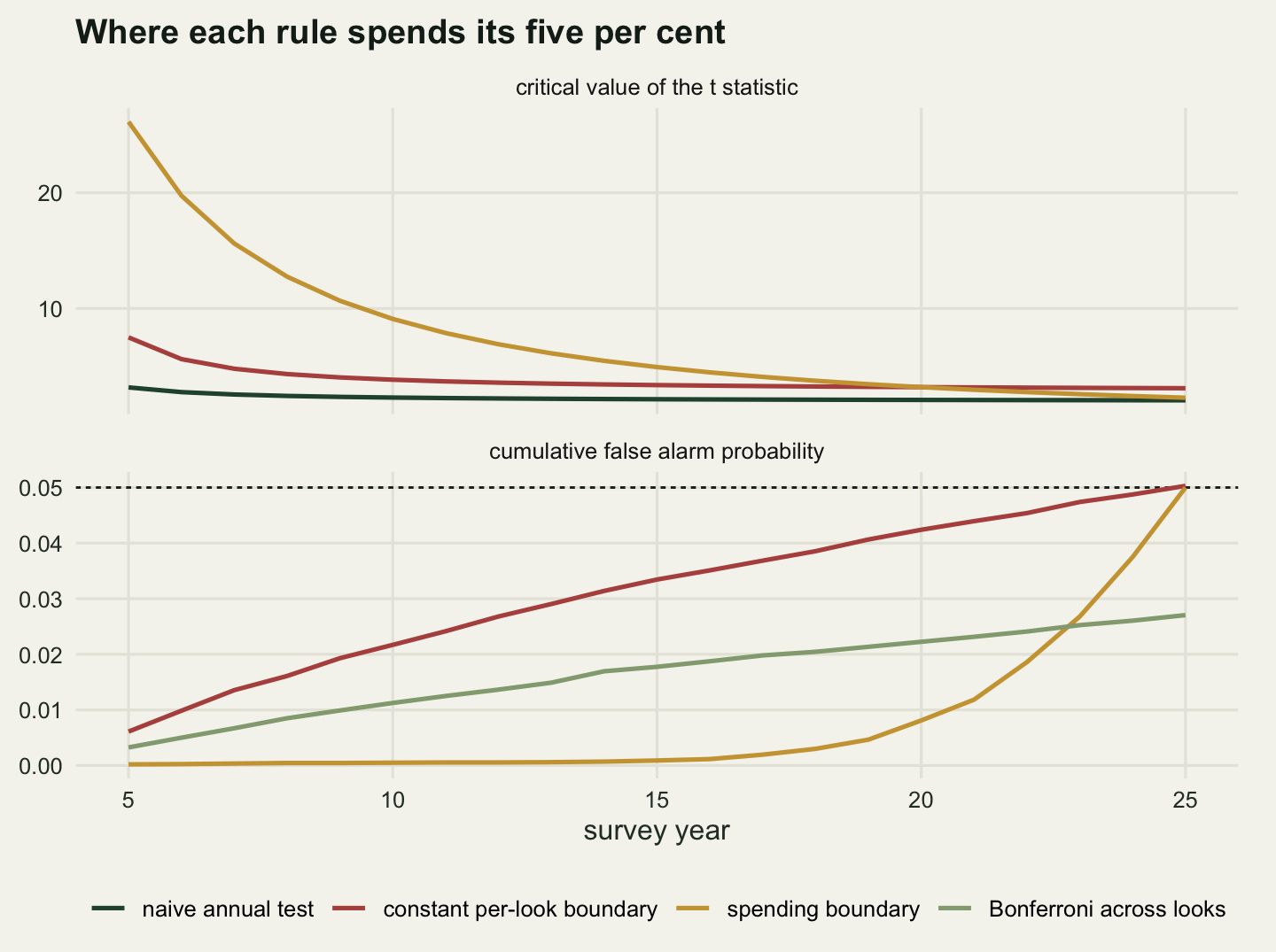
spending_crit 26.1334 15.6177 9.0985 4.9388 3.2047 2.2921The constant boundary needs a per-look level of 0.0049, which brings the overall rate to 0.0503. That is a tenth of the nominal level at every single look, and it is the honest price of asking the question twenty-one times. On the t scale it means a critical value of 3.113 at the final look instead of the usual 2.069.
The spending boundary is calibrated at 2.2921, and because the information fraction at year 5 is only 0.0077, the boundary there sits at 26.1 on the t scale, a value the data will essentially never reach. Half the information in a twenty-five year trend test arrives after year 19, which is the cubic growth of the year spread showing up in a place where it is easy to miss.
cum_poc <- cum_hit(cross_poc)
cum_of <- cum_hit(cross_of)
cum_bonf <- cum_hit(nul$p < a_bonf)
spent20 <- function(v) v[looks == 20]
print(round(rbind(year = looks, naive = cum_naive, bonferroni = cum_bonf,
                  constant = cum_poc,
                  spending = cum_of)[, c(1, 3, 6, 11, 16, 21)], 4))
[,1] [,2] [,3] [,4] [,5] [,6]
year 5.0000 7.0000 10.0000 15.0000 20.0000 25.0000
naive 0.0498 0.1076 0.1734 0.2470 0.3003 0.3430
bonferroni 0.0032 0.0067 0.0112 0.0177 0.0222 0.0271
constant 0.0061 0.0136 0.0217 0.0334 0.0424 0.0503
spending 0.0002 0.0004 0.0005 0.0009 0.0081 0.0500print(round(c(constant_spent_by_year_20 = spent20(cum_poc),
spending_spent_by_year_20 = spent20(cum_of),
constant_share_by_20 = spent20(cum_poc) / alpha_nom,
spending_share_by_20 = spent20(cum_of) / alpha_nom), 4))constant_spent_by_year_20 spending_spent_by_year_20 constant_share_by_20
0.0424 0.0081 0.8480
spending_share_by_20
0.1620 By year twenty the constant boundary has already used 0.0424 of its five per cent, or 84.8 per cent of the budget, while the spending boundary has used 0.0081, or 16.2 per cent. Everything the spending boundary has left, it spends in the last five years, which is where the information is.
What the two fixes cost against a real decline
A correction that nobody can afford is not a correction. The same three rules, plus Bonferroni and plus the fixed-horizon test at year twenty-five, now run on programmes whose population really is declining at a log-scale rate of -0.015 per year.
alt_t <- abs(qt(alt$p / 2, matrix(looks - 2, n_rep, n_look, byrow = TRUE)))
rule_row <- function(cross) {
  ix <- max.col(cross, "first")
  hit <- rowSums(cross) > 0
  sl <- alt$slope[cbind(seq_len(n_rep), ix)][hit]
  c(power = mean(hit), mc_se = sqrt(mean(hit) * (1 - mean(hit)) / n_rep),
    mean_year = mean(looks[ix][hit]), median_year = median(looks[ix][hit]),
    mean_estimate = mean(sl), bias_factor = mean(sl) / alt_slope)
}
price <- rbind(
  naive_annual = rule_row(alt$p < alpha_nom),
  bonferroni = rule_row(alt$p < a_bonf),
  constant = rule_row(alt$p < a_poc),
  spending = rule_row(alt_t > rep(of_bound(c_of), each = n_rep)),
  fixed_at_25 = rule_row(cbind(matrix(FALSE, n_rep, n_look - 1),
                               alt$p[, n_look] < alpha_nom)))
print(round(price, 4))
power mc_se mean_year median_year mean_estimate bias_factor
naive_annual 0.9295 0.0018 15.0672 15 -0.0262 1.7480
bonferroni 0.5204 0.0035 20.3117 21 -0.0235 1.5692
constant 0.6346 0.0034 19.5420 21 -0.0237 1.5827
spending 0.8310 0.0026 21.6832 22 -0.0183 1.2186
fixed_at_25 0.8640 0.0024 25.0000 25 -0.0161 1.0727print(round(c(power_lost_constant = price["naive_annual", "power"] -
price["constant", "power"],
power_lost_spending = price["naive_annual", "power"] -
price["spending", "power"],
spending_over_fixed = price["spending", "power"] /
price["fixed_at_25", "power"],
years_later_spending = price["spending", "mean_year"] -
price["constant", "mean_year"]), 4)) power_lost_constant power_lost_spending spending_over_fixed
0.2948 0.0985 0.9617
years_later_spending
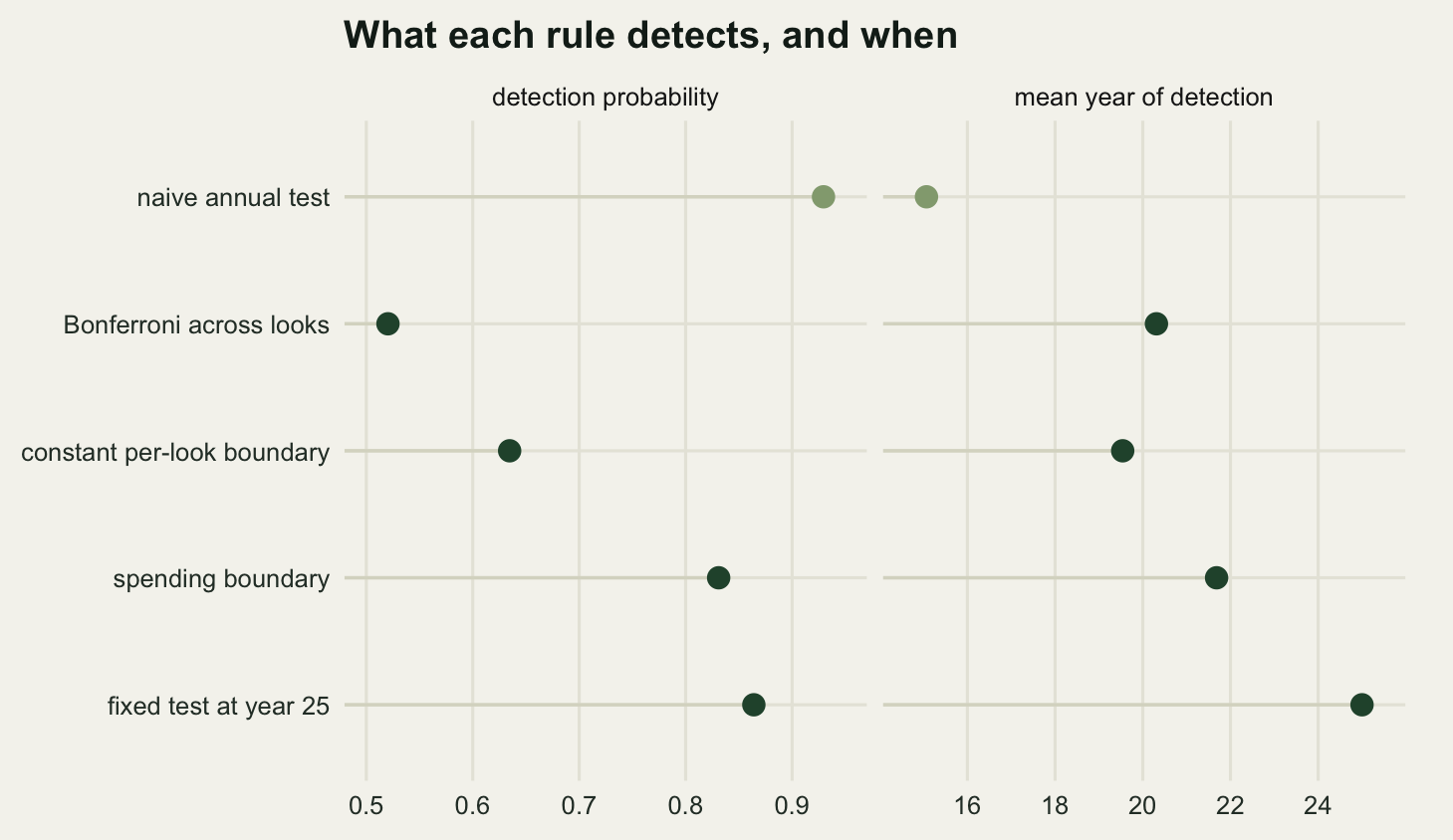
2.1411 The naive annual test detects the decline in 0.9295 of programmes, on average in year 15.07. That number is not a power, because the same rule fires in 0.343 of flat populations; it is what a procedure achieves when it is allowed to run at nearly seven times its stated error rate.
The constant boundary brings the error rate back to 0.0503 and detection falls to 0.6346, a loss of 0.2948. That is the headline cost of the repair and it is heavy: nearly a third of the detections gone, and the average detection pushed out to year 19.54.
The spending boundary does better, and this is where the shape of the information curve pays off. It detects 0.831 of true declines, which is 96.2 per cent of what the fixed-horizon test at year twenty-five achieves (0.864), while still allowing a stop at any year. It recovers 0.1963 of the 0.2948 that the constant boundary gave up. Bonferroni, the correction that felt natural, is the worst of the four: 0.5204 power for an error rate of 0.0271, which is less power than the constant boundary at 54.1 per cent of the error rate it was permitted.
Neither fix wins outright. The spending boundary wins on power and it wins on the estimate: its stopped estimate averages -0.01828 against a truth of -0.015, an inflation of 1.219, where the constant boundary gives 1.583 and the naive rule 1.748. None of them reaches the truth, and neither does the fixed-horizon test: among the year twenty-five tests that came out significant the mean estimate is 1.073 times the true value, which is the ordinary significance filter operating on its own. The constant boundary wins on speed: when it does detect, it detects in year 19.54 on average against 21.68 for the spending boundary, because it keeps a real, if small, chance of stopping at any point while the spending boundary is unreachable for the first two thirds of the study. If a programme’s reason for testing annually is that an early answer would change management, that difference of 2.14 years is the thing being bought, and the power is the thing being sold.
What an honest report looks like without a plan
Most programmes reading this will already have taken their looks, without a boundary and without recording how many. The question is what can be written up.
ix_alt <- max.col(alt$p < alpha_nom, "first")
se_stop <- alt$se[cbind(seq_len(n_rep), ix_alt)][alt_hit]
sl_stop <- alt$slope[cbind(seq_len(n_rep), ix_alt)][alt_hit]
crit_stop <- qt(0.975, looks[ix_alt][alt_hit] - 2)
cov_stop <- mean(abs(sl_stop - alt_slope) < crit_stop * se_stop)
cov_fixed <- mean(abs(alt$slope[, n_look] - alt_slope) <
                    qt(0.975, n_year - 2) * alt$se[, n_look])

print(round(c(coverage_of_naive_ci_at_stopping = cov_stop,
              coverage_at_fixed_horizon = cov_fixed,
              mean_half_width_at_stopping = mean(crit_stop * se_stop),
              mean_half_width_at_year_25 = mean(qt(0.975, n_year - 2) *
                                                  alt$se[, n_look])), 4))
coverage_of_naive_ci_at_stopping coverage_at_fixed_horizon
0.9094 0.9510
mean_half_width_at_stopping mean_half_width_at_year_25
0.0265 0.0096 print(round(c(median_stopping_year = median(looks[ix_alt][alt_hit]),
share_stopping_before_year_15 =
mean(looks[ix_alt][alt_hit] < 15)), 4)) median_stopping_year share_stopping_before_year_15
15.0000 0.4456 The nominal ninety-five per cent interval, computed at the stopping look and read at face value, covers the truth 90.94 per cent of the time against 95.1 per cent at the fixed horizon. That undercoverage is mild compared with the bias in the point estimate, and the reason is the width: the interval at stopping is 2.78 times as wide as the one at year twenty-five, wide enough to absorb most of an estimate that is 1.75 times too steep. Under a true trend of zero the same interval covers the truth in none of the stopped programmes, by construction: the interval excludes zero exactly when the test was significant, which is exactly when the programme stopped.
So the report can carry the estimate and the interval, and it should carry two more things. The number of looks taken, because a p value from an unplanned look is not interpretable at face value and a reader who knows there were twenty-one of them can price it. And the estimate at the full horizon alongside the one at the stopping look, if the counting continued, because they are answers to different questions and the difference between them is the size of the selection effect in that particular programme.
The honest limit
Every boundary above assumes the number and the timing of the looks were fixed before the first count. A monitoring programme almost never knows how long it will run. Funding arrives in three-year blocks, a reserve changes hands, a species gets listed and the survey suddenly matters. The calibration depends on the schedule, and not weakly.
sched <- t(vapply(c(1, 2, 5), function(step) {
  jx <- which((looks - k_min) %% step == 0)
  c(gap_years = step, looks = length(jx),
    type1 = mean(rowSums(nul$p[, jx, drop = FALSE] < alpha_nom) > 0),
    power = mean(rowSums(alt$p[, jx, drop = FALSE] < alpha_nom) > 0))
}, numeric(4)))
print(round(sched, 4))
gap_years looks type1 power
[1,] 1 21 0.3430 0.9295
[2,] 2 11 0.2818 0.9164
[3,] 5 5 0.1935 0.8972Testing every year gives an error rate of 0.343, every second year 0.2818, every fifth year 0.1935. A boundary calibrated for five looks and then used for twenty-one is not a correction, it is a different, smaller mistake. The spending-function form of Lan and DeMets (1983) exists for exactly this reason: it fixes the shape of the spending against information rather than against a list of dates, so a look inserted because a funder asked for one does not invalidate what came before. Adopting it means writing the spending function into the monitoring protocol, in the same document that fixes the plot locations.
Two further limits. The boundaries assume a stable observation process, and a programme that changes method part-way through has a different and worse problem: a step in the index reads as trend whether or not anybody tests annually, and the post on splicing a monitoring series measures that separately. And everything here controls an error rate for one hypothesis about one population; a scheme that tests fifty species every year has both this problem and the ordinary multiple-comparison problem, and the two corrections do not compose by multiplying them together.
The deepest limit is that a corrected test still answers a hypothesis question. Nichols and Williams (2006) argue that monitoring earns its cost only when it is tied to a decision, and Legg and Nagy (2006) make the same point about programmes designed without a stated question and without the power to answer it. Whether to move the grazing, fence the site or write the species off is priced by the loss of acting late against the cost of acting early, not by an alpha level. A boundary stops a programme from fooling itself; it does not tell it what to do.
Where to go next
If the reason for testing every year is that the answer would change management, the sequential decision problem is the better formulation, and when to stop monitoring sets it up as one. If the question is how long the scheme has to run before it can see the decline it cares about, that is fixed-horizon power, and it is worth doing before the boundary is chosen, because a spending boundary on a series with no power to begin with just moves the failure later. And if the scheme carries many species rather than one, the corrections across hypotheses in the multiple-testing series apply on top of this one rather than instead of it.
The practical version is short. Decide the shape of the spending function when the protocol is written; record every look, including the ones that came to nothing; and when a look does cross, report the estimate knowing that it is the steepest version of the truth the programme was ever going to see.
References
Armitage P, McPherson CK, Rowe BC 1969 Journal of the Royal Statistical Society Series A 132(2):235-244 (10.2307/2343787)
Pocock SJ 1977 Biometrika 64(2):191-199 (10.1093/biomet/64.2.191)
O’Brien PC, Fleming TR 1979 Biometrics 35(3):549-556 (10.2307/2530245)
Lan KKG, DeMets DL 1983 Biometrika 70(3):659-663 (10.1093/biomet/70.3.659)
Whitehead J 1986 Biometrika 73(3):573-581 (10.1093/biomet/73.3.573)
Jennison C, Turnbull BW 2000 Group Sequential Methods with Applications to Clinical Trials (ISBN 978-0849303166)
Nichols JD, Williams BK 2006 Trends in Ecology and Evolution 21(12):668-673 (10.1016/j.tree.2006.08.007)
Legg CJ, Nagy L 2006 Journal of Environmental Management 78(2):194-199 (10.1016/j.jenvman.2005.04.016)
Simmons JP, Nelson LD, Simonsohn U 2011 Psychological Science 22(11):1359-1366 (10.1177/0956797611417632)