---
title: "Power to detect a population trend"
description: "Turn monitoring variance components into statistical power in R, and why extra years buy far more than extra sites, with a ceiling no sample size removes."
date: "2026-06-26 11:00"
date-modified: "2026-10-14"
categories: [R, survey design, monitoring, ecology tutorial]
image: thumbnail.png
image-alt: "Power curves against number of monitoring years for several sample sizes, all converging on a single ceiling curve"
---
*Corrected 14 October 2026: the caption of the power figure put the horizontal gap between the curves at about a year; it now says that the outermost curves are about two years apart at the eighty per cent line.*
*Corrected 1 October 2026: the post called the simulated three per cent decline invisible to a ten year programme at thirty sites, beside a power showing that some such programmes would detect it; it now says most such programmes would miss it.*
*Corrected 30 September 2026: the post said that one extra year beats unlimited sites across the whole grid; that holds for the larger site designs, and the text now says that for the smallest design measuring every site wins.*
A monitoring programme is often justified with a sentence like "we will be able to detect a decline". Whether that is true is a calculation, it needs three inputs, and all three can be pinned down before the full programme starts: the variance components (from a pilot or a comparable programme), the design, and the size of the change worth detecting.
This post does the calculation for a programme that revisits the same sites, checks it against simulation, and then asks the question that decides most monitoring budgets. Given a fixed amount of money, is it better spent on more sites or on more years?
## From variance components to a standard error
The trend comes from a regression of the annual means on year. Its variance was derived in the first post of this series: the year component enters undivided, the site by year and residual components are divided by the number of sites, the persistent site differences drop out entirely, and the whole thing is divided by the spread of the year index.
```{r se-function}
sd_site <- 0.55; sd_year <- 0.20; sd_sy <- 0.30; sd_res <- 0.35
n_rep <- 2                       # counts per site visit

se_trend <- function(n_year, n_site, k = n_rep) {
  Sxx <- n_year * (n_year^2 - 1) / 12          # sum of squares of the centred year index
  sqrt((sd_year^2 + (sd_sy^2 + sd_res^2 / k) / n_site) / Sxx)
}

data.frame(years = c(10, 10, 10, 20),
           sites = c(10, 30, 100, 30),
           se    = round(se_trend(c(10, 10, 10, 20), c(10, 30, 100, 30)), 5))
```
Two features of that expression decide everything below. The site count divides only part of the numerator, so its effect saturates. The year count enters through `Sxx`, which grows with the cube of the number of years, so the standard error falls like the number of years to the power of one and a half.
## The power calculation
With the standard error in hand, power is the probability that a two-sided test rejects a zero trend when the true trend is not zero. The test statistic follows a non-central t distribution with the degrees of freedom of the annual-mean regression.
```{r power-function}
trend_power <- function(n_year, n_site, beta, alpha = 0.05, k = n_rep) {
  df   <- n_year - 2
  ncp  <- abs(beta) / se_trend(n_year, n_site, k)
  crit <- qt(1 - alpha / 2, df)
  pt(-crit, df, ncp) + (1 - pt(crit, df, ncp))
}
beta_true <- -0.03               # about 3 per cent a year on the log scale
round(trend_power(c(10, 15, 20, 25), 30, beta_true), 3)
```
Before that function is trusted, it is worth running the programme it describes.
```{r power-mc}
sim_programme <- function(n_year, n_site, beta) {
  s  <- rnorm(n_site, 0, sd_site)
  a  <- rnorm(n_year, 0, sd_year)
  tc <- (1:n_year) - mean(1:n_year)
  annual <- vapply(1:n_year, function(j) {
    mean(3 + beta * tc[j] + s + a[j] + rnorm(n_site, 0, sd_sy) +
         rnorm(n_site, 0, sd_res / sqrt(n_rep)))
  }, numeric(1))
  co <- summary(lm(annual ~ tc))$coefficients[2, ]
  abs(co[1] / co[2]) > qt(0.975, n_year - 2)
}

set.seed(369)
mc_power <- mean(replicate(3000, sim_programme(15, 30, beta_true)))
c(simulated = mc_power, formula = trend_power(15, 30, beta_true))
```
Simulated power `r sprintf("%.3f", mc_power)` against a formula value of `r sprintf("%.3f", trend_power(15, 30, beta_true))`, from `r format(3000, big.mark = ",")` simulated programmes. The formula can be used.
## Years beat sites
Here is the same calculation across a grid of designs. The last column is the limit as the number of sites goes to infinity, which is a real ceiling rather than a rhetorical one: it is the power a programme would have with every site in the region measured, every year, perfectly.
```{r power-grid}
years <- c(10, 12, 15, 20, 25)
sites <- c(10, 30, 100, 1e6)
grid <- outer(years, sites, Vectorize(function(y, n) trend_power(y, n, beta_true)))
dimnames(grid) <- list(paste(years, "years"), c("10 sites", "30 sites", "100 sites", "all sites"))
round(grid, 3)
```
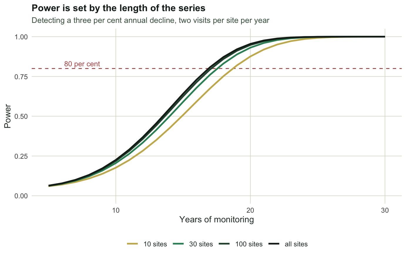
Read along the first row. Ten years of 30 sites gives power `r sprintf("%.3f", trend_power(10, 30, beta_true))`. Tripling to 100 sites gives `r sprintf("%.3f", trend_power(10, 100, beta_true))`. Measuring the entire region gives `r sprintf("%.3f", trend_power(10, max(sites), beta_true))`. Now go down the second column instead: adding a single year to the original design (11 years, which falls between the first two rows of the table) gives `r sprintf("%.3f", trend_power(11, 30, beta_true))`.
**One extra year is worth more than an unlimited number of extra sites.** That is not a rounding artefact, and it holds at every series length in the grid for the 30- and 100-site designs. With only ten sites it fails: there the site-level noise is still large enough that measuring every site beats one extra year.
```{r fig-power}
#| echo: false
#| fig-width: 7.2
#| fig-height: 4.6
#| fig-cap: "Power to detect a three per cent annual decline, against the length of the monitoring series. The four curves are 10, 30 and 100 sites and the limit of infinitely many sites. They are close together and far apart in the wrong direction: at the eighty per cent line the outermost curves are about two years apart, while a year of extra data moves a programme up the curve."
#| fig-alt: "Four rising S-shaped power curves against years of monitoring, packed close together, crossing the eighty per cent line between seventeen and nineteen years."
library(ggplot2)
theme_te <- function(base_size = 11) {
theme_minimal(base_size = base_size) +
theme(plot.background = element_rect(fill = "#f5f4ee", colour = NA),
panel.background = element_rect(fill = "#f5f4ee", colour = NA),
panel.grid.minor = element_blank(),
panel.grid.major = element_line(colour = "#dad9ca", linewidth = 0.3),
text = element_text(colour = "#2c3a31"),
plot.title = element_text(colour = "#16241d", face = "bold", size = base_size + 1),
plot.subtitle = element_text(colour = "#46604a", size = base_size - 1))
}
yy <- 5:30
curves <- do.call(rbind, lapply(c(10, 30, 100, 1e6), function(n) {
data.frame(years = yy, power = trend_power(yy, n, beta_true),
sites = if (n > 1e5) "all sites" else paste(n, "sites"))
}))
curves$sites <- factor(curves$sites, levels = c("10 sites", "30 sites", "100 sites", "all sites"))
ggplot(curves, aes(years, power, colour = sites)) +
geom_hline(yintercept = 0.8, linetype = "dashed", colour = "#b5534e") +
geom_line(linewidth = 1) +
annotate("text", x = 7.5, y = 0.83, label = "80 per cent", colour = "#b5534e", size = 3.2) +
scale_colour_manual(values = c("#c9b458", "#2f8f63", "#275139", "#16241d")) +
scale_y_continuous(limits = c(0, 1)) +
labs(x = "Years of monitoring", y = "Power", colour = NULL,
title = "Power is set by the length of the series",
subtitle = "Detecting a three per cent annual decline, two visits per site per year") +
theme_te() + theme(legend.position = "bottom")
```
The same point in units a budget holder understands. How many years does each design need before it reaches 80 per cent power?
```{r years-to-80}
years_to_80 <- function(n_site, beta = beta_true) {
  y <- 5:40
  y[which(trend_power(y, n_site, beta) >= 0.8)[1]]
}
data.frame(sites = c(10, 30, 100, 1000, 1e6),
           years_needed = sapply(c(10, 30, 100, 1000, 1e6), years_to_80))
```
Ten sites need `r years_to_80(10)` years and the whole region needs `r years_to_80(1e6)`. Every site that exists, measured perfectly, saves `r years_to_80(10) - years_to_80(1e6)` years against a programme with ten sites.
## Where the ceiling comes from
The two levers are not the same shape.
```{r levers}
c(double_the_sites = se_trend(15, 30) / se_trend(15, 60),
  double_the_years = se_trend(15, 30) / se_trend(30, 30),
  three_halves_rule = 2^1.5)
```
Doubling the sites from 30 to 60 divides the standard error by `r sprintf("%.3f", se_trend(15, 30) / se_trend(15, 60))`. Doubling the years from 15 to 30 divides it by `r sprintf("%.2f", se_trend(15, 30) / se_trend(30, 30))`, close to the two to the power of one and a half that the cubic growth of `Sxx` predicts.
The reason sits in the year component. A year effect is shared by every site in the region, so averaging over sites does not reduce it: a warm spring lifts all the counts at once, and 10,000 sites see the same warm spring as 10 sites. Only more years can average it away, and more years also stretch the lever arm of the regression. That is why the two levers differ by an order of magnitude.
## What a programme can honestly promise
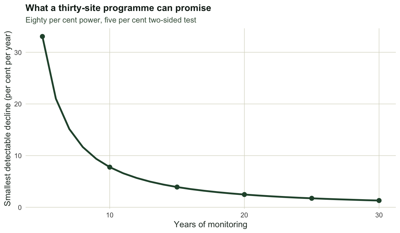
Turn the question round. Given a design, what is the smallest trend it can detect with 80 per cent power?
```{r detectable}
detectable <- function(n_year, n_site, power = 0.8, alpha = 0.05) {
  f <- function(b) trend_power(n_year, n_site, b, alpha) - power
  uniroot(f, c(1e-5, 1))$root
}
tab <- data.frame(years = c(5, 10, 15, 20, 25),
                  sites = 30)
tab$detectable_log <- sapply(tab$years, detectable, n_site = 30)
tab$decline_per_cent <- 100 * (1 - exp(-tab$detectable_log))   # a fall, not a rise
tab$half_in_years <- log(2) / tab$detectable_log
data.frame(years = tab$years, sites = tab$sites,
           detectable_log = round(tab$detectable_log, 4),
           decline_per_cent = round(tab$decline_per_cent, 1),
           half_in_years = round(tab$half_in_years, 1))
```
```{r fig-detectable}
#| echo: false
#| fig-width: 7.2
#| fig-height: 4.2
#| fig-cap: "The smallest annual decline a 30-site programme can detect with 80 per cent power, against the length of the series. A five year programme can only see a collapse; a twenty year programme can see a change slow enough to matter for management."
#| fig-alt: "Steeply falling curve from about twenty-five per cent per year at five years down to under one and a half per cent per year at thirty years, with points marked at five year intervals."
dd <- data.frame(years = 5:30)
dd$pct <- 100 * (1 - exp(-sapply(dd$years, detectable, n_site = 30)))
ggplot(dd, aes(years, pct)) +
geom_line(colour = "#275139", linewidth = 1.1) +
geom_point(data = dd[dd$years %% 5 == 0, ], colour = "#275139", size = 2.4) +
labs(x = "Years of monitoring", y = "Smallest detectable decline (per cent per year)",
title = "What a thirty-site programme can promise",
subtitle = "Eighty per cent power, five per cent two-sided test") +
theme_te()
```
A ten year programme at 30 sites can detect a decline of `r sprintf("%.1f", 100 * (1 - exp(-detectable(10, 30))))` per cent a year, which is a population halving in `r sprintf("%.1f", log(2) / detectable(10, 30))` years. The three per cent decline this series has been simulating would be missed by most programmes of that design: power `r sprintf("%.2f", trend_power(10, 30, beta_true))`. At twenty years the same programme reaches `r sprintf("%.1f", 100 * (1 - exp(-detectable(20, 30))))` per cent a year.
This is the number that belongs in a monitoring proposal, and it is rarely there. "We will detect declines" is not a claim until the sentence names a size and a horizon.
Two honest limits before this is used in anger. The calculation assumes a linear trend on the log scale, tested at the end of a fixed period; a programme analysed every year with the same test has a multiple testing problem that this power number does not cover. And every input is an estimate, usually from a short pilot. The next post measures how much that second point matters, and it is more than one would guess.
## Where this leaves the series
Power is the promise a monitoring programme makes to whoever funds it. It comes from three numbers, two of which are decided at the design stage and one of which is inherited from the ecology. The closing post of this series checks the promise from three directions.
## References
Gerrodette 1987 Ecology 68(5):1364-1372 (10.2307/1939220)
Urquhart, Paulsen and Larsen 1998 Ecological Applications 8(2):246-257 (10.1890/1051-0761(1998)008[0246:MFPRRO]2.0.CO;2)
Rhodes and Jonzen 2011 Ecography 34(6):1040-1048 (10.1111/j.1600-0587.2011.06370.x)
Larsen, Kincaid, Jacobs and Urquhart 2001 BioScience 51(12):1069-1078 (10.1641/0006-3568(2001)051[1069:DFELAR]2.0.CO;2)
## Related tutorials
- [Variance components in monitoring data](../variance-components-in-monitoring/)
- [Revisit designs for long-term monitoring](../revisit-designs-for-monitoring/)
- [Checking a monitoring design](../checking-a-monitoring-design/)
- [Taylor's power law and how many quadrats](../taylors-power-law-and-sample-size/)