library(ggplot2)

te_paper  <- "#f5f4ee"
te_ink    <- "#16241d"
te_body   <- "#2c3a31"
te_forest <- "#275139"
te_rust   <- "#b5534e"
te_gold   <- "#c9b458"
te_line   <- "#dad9ca"

theme_datasheet <- function() {
  theme_minimal(base_size = 12) +
    theme(plot.background  = element_rect(fill = te_paper, colour = NA),
          panel.background = element_rect(fill = te_paper, colour = NA),
          panel.grid.major = element_line(colour = te_line, linewidth = 0.3),
          panel.grid.minor = element_blank(),
          text             = element_text(colour = te_body),
          plot.title       = element_text(colour = te_ink, face = "bold"),
          axis.text        = element_text(colour = te_body))
}Taylor’s power law and how many quadrats
R
sampling design
count data
spatial ecology
ecology tutorial
Variance scales with the mean as a power law, and the exponent prices a survey. Fit it in R, turn it into quadrat counts, and watch it move with grain.
Corrected 7 October 2026: the post said the coarsest grain returns the least stable exponent of the four, a ranking that a hundred repeats cannot settle against the one metre grain; it now compares the coarsest grain only with the finest.
Corrected 30 September 2026: the post said a Taylor slope near one shows only that counts behaved like independent draws, and that the one metre grain returns the noisier exponent; it now says a slope of one needs an intercept near one as well to match independent counts, and that the gap in stability between the one and two metre grains is within Monte Carlo error.
A survey plan comes down to one number: how many quadrats. The usual way to get it is to run a pilot, take the variance of the pilot counts, and put it in the formula for the standard error of a mean. That works for the density the pilot happened to have and nowhere else, because the variance of a count is not a property of the sampling design. It is a function of the mean, and the function is a power.
Taylor’s power law says the variance across a set of samples scales as a power of their mean. It usually appears in this literature as a diagnostic: fit the log-log slope, see whether it exceeds one, conclude that the counts are aggregated. That reading throws away the useful half. The fitted power is a price list. It converts a target precision into a number of quadrats at any density, it says how that number changes when the population thins out, and it is the thing a survey design has to pay for. This post fits the law, turns it into quadrats, checks the arithmetic against a direct simulation of the sampling distribution, and then shows the grain problem that stops the answer transferring between studies.
The law and its Poisson null
The statement is short. Take a set of populations, or one population at a set of sites, dates or densities. For each, compute the mean count per quadrat and the variance of the counts across quadrats. Then variance and mean are tied by
V = a * M^b
with the exponent b estimated as the slope of log(V) on log(M). The generator below produces counts with exactly that relationship, by solving the negative binomial size parameter from the target variance at each mean. When the target variance falls to the mean itself, the size parameter goes to infinity and the draw is Poisson, so the same function covers the null.
rcount <- function(nq, M, a, b) {
  vtarget <- a * M^b
  if (vtarget <= M * 1.000001) return(rpois(nq, M))
  rnbinom(nq, mu = M, size = M^2 / (vtarget - M))
}

fit_law <- function(counts) {
  m  <- colMeans(counts)
  v  <- apply(counts, 2, var)
  ok <- m > 0 & v > 0
  f  <- lm(log(v[ok]) ~ log(m[ok]))
  c(a = unname(exp(coef(f)[1])), b = unname(coef(f)[2]), sites = sum(ok))
}

M_site <- exp(seq(log(0.4), log(45), length.out = 40))
n_q    <- 25
a_true <- 2.4
b_true <- 1.55

set.seed(20260813)
counts_pois <- sapply(M_site, function(m) rpois(n_q, m))
set.seed(20260813)
counts_clus <- sapply(M_site, function(m) rcount(n_q, m, a_true, b_true))

law_pois <- fit_law(counts_pois)
law_clus <- fit_law(counts_clus)
round(rbind(Poisson = law_pois, clustered = law_clus), 3)
a b sites
Poisson 0.983 0.985 40
clustered 2.323 1.479 40Forty sites, 25 quadrats at each, means running from 0.4 to 45 individuals per quadrat. The two data sets share the seed and the site means, and the variance rule is the only thing that differs between the two generators. They are not matched draw for draw, because rpois and rnbinom take different amounts from the random stream.
Independent counts give b of 0.98 and a of 0.98 here, against the exact Poisson values of one and one. That is the negative control the fitted exponent needs, and it is worth running before any interpretation: a slope near one together with an intercept near one is what independent draws give, but a slope near one on its own does not show independence, because counts whose variance is a fixed multiple of the mean also return a slope of one. The clustered set returns b of 1.48 and a of 2.32 against generating values of 1.55 and 2.4.
law_df <- rbind(
  data.frame(mean_count = colMeans(counts_pois),
             variance   = apply(counts_pois, 2, var), counts = "independent"),
  data.frame(mean_count = colMeans(counts_clus),
             variance   = apply(counts_clus, 2, var), counts = "clustered"))
law_df$counts <- factor(law_df$counts, levels = c("clustered", "independent"))

ggplot(law_df, aes(mean_count, variance, colour = counts)) +
  geom_abline(slope = 1, intercept = 0, linetype = "dashed", colour = te_body) +
  geom_point(size = 2.2) +
  geom_abline(slope = law_clus["b"], intercept = log10(law_clus["a"]),
              colour = te_rust, linewidth = 0.9) +
  geom_abline(slope = law_pois["b"], intercept = log10(law_pois["a"]),
              colour = te_forest, linewidth = 0.9) +
  scale_x_log10() + scale_y_log10() +
  scale_colour_manual(values = c(te_rust, te_forest)) +
  labs(x = "mean count per quadrat", y = "variance across quadrats",
       colour = NULL, title = "One slope, and the null it is measured against") +
  theme_datasheet() +
  theme(legend.position = "bottom")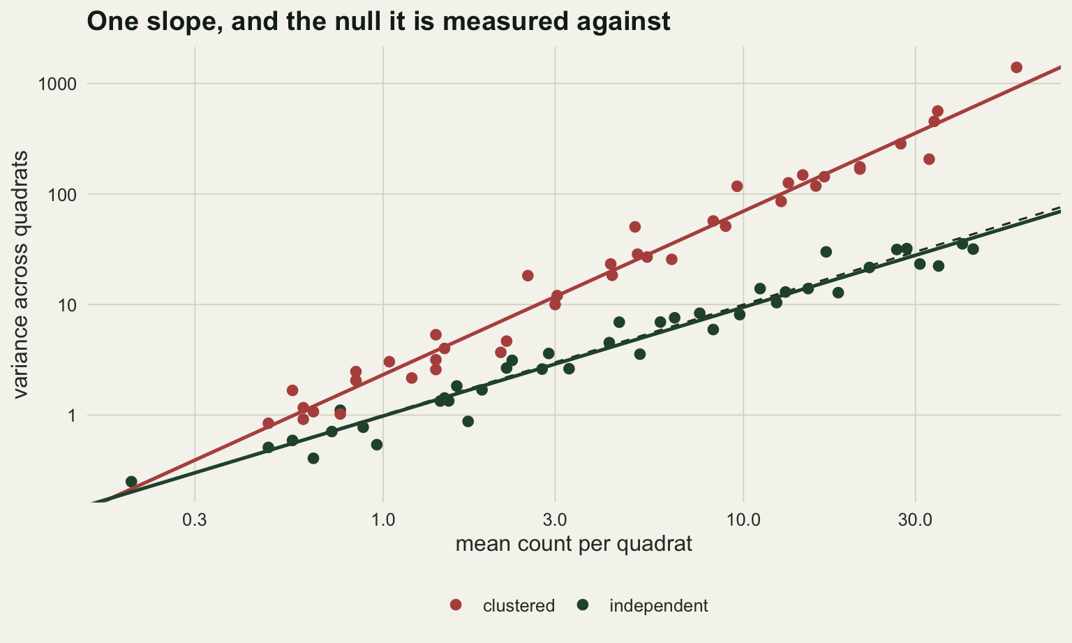
The dashed line is the Poisson case. Everything above it costs more quadrats than a Poisson calculation would predict, and the gap widens with density because the two lines have different slopes, not just different heights.
What the law costs in quadrats
Here is the whole payment, in two lines. The mean of n quadrats drawn at random from a population with mean M and per-quadrat variance V has variance V / n, so its standard error is sqrt(V / n). Substituting the power law and dividing by M to get the relative standard error,
RSE = sqrt(a * M^(b - 2) / n)
and rearranging for the sample size that hits a target RSE,
n = a * M^(b - 2) / RSE^2
That is Karandinos’ formula, in the form that appears throughout the applied sampling literature. Two features of it are worth more than the algebra. The exponent enters as b - 2, not b, so the quantity that decides how sample size responds to density is the distance of the exponent from two. And a and b come from a fitted line, so the number of quadrats inherits whatever error that line carries.
The formula is a claim about the sampling distribution of a mean, so it can be checked against one directly. For four densities, take the n it prescribes for a twenty per cent relative standard error, draw four thousand surveys of that size, and compare the spread of the resulting means with what the formula predicts at that rounded n.
n_quadrats <- function(M, a, b, rse) a * M^(b - 2) / rse^2

rse_target <- 0.20
M_check    <- c(0.5, 2, 10, 40)
n_rep      <- 4000
mc_se      <- rse_target / sqrt(2 * (n_rep - 1))

set.seed(4747)
cost_tab <- do.call(rbind, lapply(M_check, function(m) {
  nq     <- ceiling(n_quadrats(m, a_true, b_true, rse_target))
  survey <- replicate(n_rep, mean(rcount(nq, m, a_true, b_true)))
  data.frame(mean_count  = m,
             quadrats    = nq,
             formula_rse = sqrt(a_true * m^(b_true - 2) / nq),
             simulated_rse = sd(survey) / m)
}))
print(cost_tab, row.names = FALSE, digits = 3)
mean_count quadrats formula_rse simulated_rse
0.5 82 0.200 0.197
2.0 44 0.200 0.204
10.0 22 0.197 0.201
40.0 12 0.195 0.194The prescribed sample sizes are 82, 44, 22, 12 quadrats for mean counts of 0.5, 2, 10, 40 per quadrat. The formula’s relative standard error and the one measured from 4000 simulated surveys agree to 0.004 at worst, against a Monte Carlo standard error of 0.002 on each simulated value, so the largest gap is 1.8 times that noise: of the order of the Monte Carlo error of the check itself rather than inside it. The formula is not an approximation that degrades at low counts; it is exact for the standard error, and the only approximation is in reading a standard error as a precision when the sampling distribution of the mean is skewed.
The exponent sets the shape, not just the level
Now hold a fixed and vary b, which separates the two things the fitted law does. The intercept sets the level of the cost. The exponent sets how the cost responds to density, and that is the part with ecological content.
b_grid <- c(1, b_true, 2)
M_grid <- exp(seq(log(0.2), log(50), length.out = 200))
cost_df <- do.call(rbind, lapply(b_grid, function(bb)
  data.frame(mean_count = M_grid,
             quadrats   = n_quadrats(M_grid, a_true, bb, rse_target),
             exponent   = factor(sprintf("b = %.2f", bb),
                                 levels = sprintf("b = %.2f", b_grid)))))

p_cost <- ggplot(cost_df, aes(mean_count, quadrats, colour = exponent)) +
  geom_vline(xintercept = 1, linetype = "dashed", colour = te_body) +
  geom_line(linewidth = 1) +
  scale_x_log10() + scale_y_log10() +
  scale_colour_manual(values = c(te_forest, te_rust, te_gold)) +
  labs(x = "mean count per quadrat", y = "quadrats for a 20 per cent standard error",
       colour = NULL, title = "What the exponent costs at low density") +
  theme_datasheet() +
  theme(legend.position = "bottom")
p_cost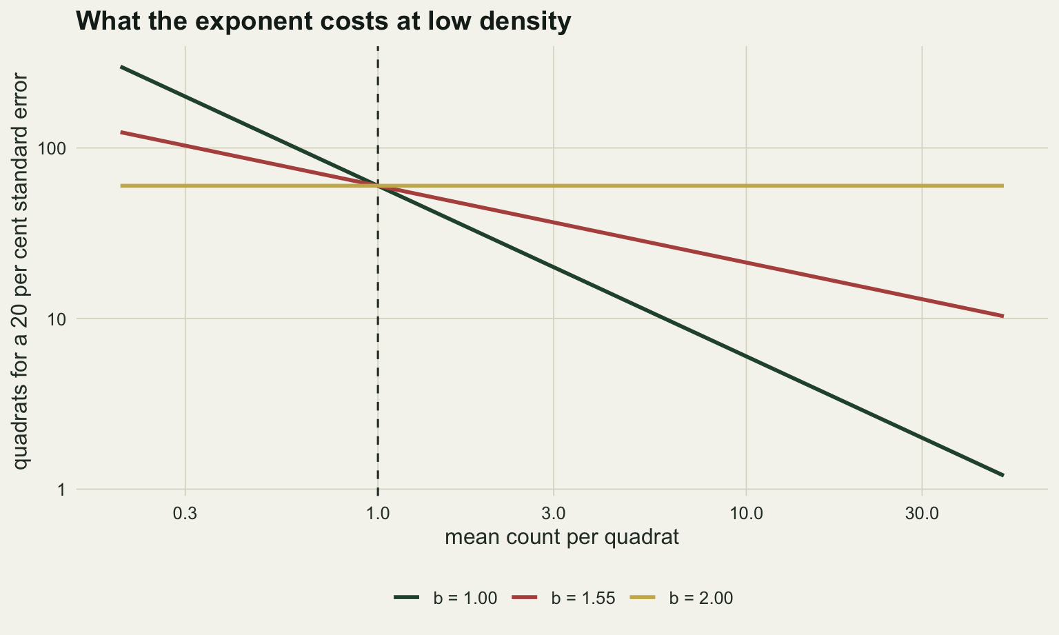
At b of two the required sample size is a / RSE^2 whatever the density, so the curve is flat and a design that works in a dense patch works unchanged in a sparse one. That is the only exponent with that property, and it is the one implicitly assumed whenever a survey is planned on a coefficient of variation rather than a variance. Below two the cost climbs as the population thins. At the Poisson exponent of one the climb is exactly proportional: a factor of ten drop in density is a factor of ten more quadrats, 120 against 12 for the two ends of that step. At 1.55 the same drop costs a factor of 2.8.
That last comparison runs the opposite way to the reflex. Aggregation raises the level of the cost at any density above one count per quadrat, but by pushing the exponent towards two it flattens the density response, so it is the near-Poisson species whose survey cost climbs fastest as it thins. That is a statement about the rate and not the level, and the difference matters because the three curves above share an intercept only because a was held fixed to isolate the exponent. Give the Poisson case the intercept it actually has, one rather than 2.4, and at half an individual per quadrat it needs 50 quadrats against the aggregated species’ 82. The steeper response still belongs to the Poisson species; the higher bill does not. The crossing point of the three lines sits at one count per quadrat because M^(b - 2) is one there, and that point is not biology. It is wherever the quadrat happens to be sized so the mean count is one, which is the subject of the next section.
The exponent moves with the quadrat size
A published b is often reused as though it belonged to the species. It does not. It belongs to the species and the quadrat, and the second half travels badly. To see how badly, the twelve fields below share one set of clump centres. Two hundred parent locations are drawn once, uniformly over a thirty two metre square, and every density level scatters a Poisson number of offspring around those same parents, each offspring displaced by an independent Gaussian with a standard deviation of one metre. Density is varied through the offspring per parent, so the clumps stay where they are and the clustering scale stays at one metre; what changes across the twelve levels is how crowded each clump is. Everything is base R; the wrap onto a torus keeps the border from being thinned.
plot_side <- 32
n_parent  <- 200

set.seed(5012)
parents <- cbind(runif(n_parent, 0, plot_side), runif(n_parent, 0, plot_side))

sim_cluster <- function(par_xy, mu_off, sigma, seed) {
  set.seed(seed)
  k <- rpois(nrow(par_xy), mu_off)
  x <- rep(par_xy[, 1], k) + rnorm(sum(k), 0, sigma)
  y <- rep(par_xy[, 2], k) + rnorm(sum(k), 0, sigma)
  cbind(x %% plot_side, y %% plot_side)
}

quad_counts <- function(pts, side) {
  g  <- round(plot_side / side)
  ix <- pmin(floor(pts[, 1] / side), g - 1)
  iy <- pmin(floor(pts[, 2] / side), g - 1)
  tabulate(ix * g + iy + 1, nbins = g * g)
}

mu_levels <- exp(seq(log(8), log(90), length.out = 12))
fields    <- lapply(seq_along(mu_levels),
                    function(i) sim_cluster(parents, mu_levels[i], 1, 5000 + i))
sides     <- c(4, 2, 1, 0.5)

grain_mv <- do.call(rbind, lapply(sides, function(s) do.call(rbind,
  lapply(fields, function(p) {
    z <- quad_counts(p, s)
    data.frame(side = s, mean_count = mean(z), variance = var(z))
  }))))

grain <- do.call(rbind, lapply(sides, function(s) {
  d <- grain_mv[grain_mv$side == s, ]
  f <- lm(log(d$variance) ~ log(d$mean_count))
  data.frame(side = s, quadrats_in_plot = (plot_side / s)^2,
             a = unname(exp(coef(f)[1])), b = unname(coef(f)[2]))
}))
print(grain, row.names = FALSE, digits = 3)
side quadrats_in_plot a b
4.0 64 0.256 1.91
2.0 256 0.574 1.85
1.0 1024 1.086 1.65
0.5 4096 1.485 1.35grain_mv$quadrat <- factor(sprintf("%.1f m", grain_mv$side),
levels = sprintf("%.1f m", sides))
grain$quadrat <- factor(sprintf("%.1f m", grain$side),
levels = sprintf("%.1f m", sides))
ggplot(grain_mv, aes(mean_count, variance, colour = quadrat)) +
geom_abline(data = grain, aes(slope = b, intercept = log10(a), colour = quadrat),
linewidth = 0.8) +
geom_point(size = 2.2) +
scale_x_log10() + scale_y_log10() +
scale_colour_manual(values = c(te_ink, te_rust, te_forest, te_gold)) +
labs(x = "mean count per quadrat", y = "variance across quadrats",
colour = "quadrat side", title = "Twelve fields, four grains, four laws") +
theme_datasheet() +
theme(legend.position = "bottom")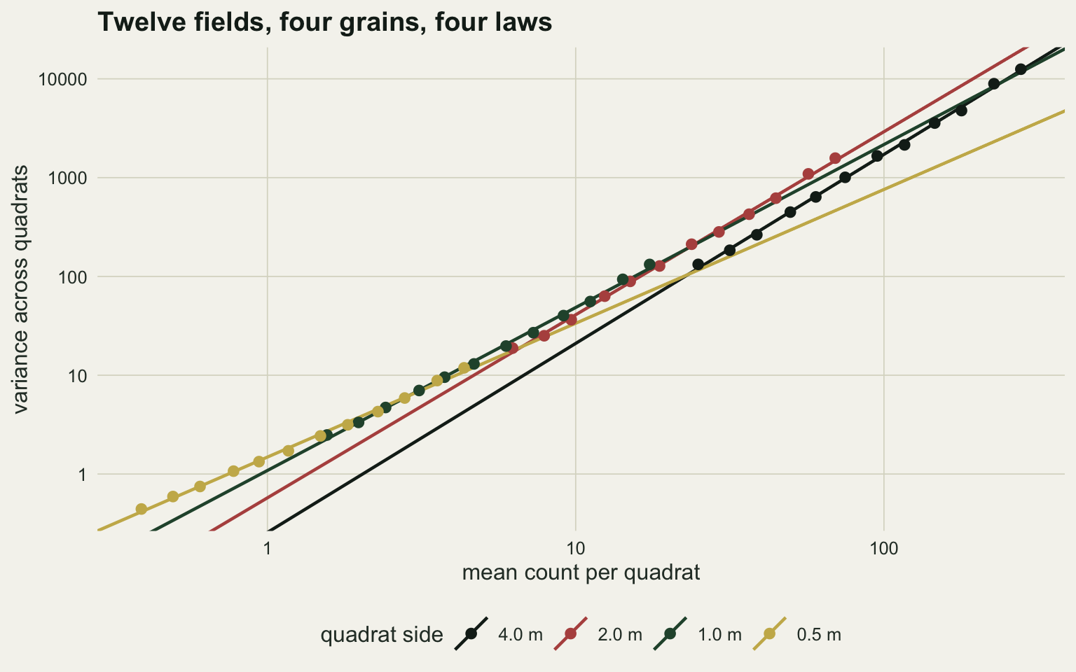
The exponent runs from 1.35 to 1.91 and the intercept from 0.26 to 1.49 across the four quadrat sizes, on twelve fields that share one set of clump centres and one clustering scale. Nothing about the organisms changed between those numbers. The ordering is a gradient: the exponent falls at every step down in quadrat size, as the quadrat side goes from four times the one metre clustering scale to half of it. That is worth checking on more than one draw, since a single fitted line per grain is itself an estimate.
grain_b <- function(seed) {
  set.seed(seed)
  pp <- cbind(runif(n_parent, 0, plot_side), runif(n_parent, 0, plot_side))
  fs <- lapply(seq_along(mu_levels),
               function(i) sim_cluster(pp, mu_levels[i], 1, seed * 100 + i))
  sapply(sides, function(s) {
    d <- do.call(rbind, lapply(fs, function(p) {
      z <- quad_counts(p, s)
      c(mean(z), var(z))
    }))
    unname(coef(lm(log(d[, 2]) ~ log(d[, 1])))[2])
  })
}

reps <- t(sapply(1:100, function(r) grain_b(70000 + r)))
colnames(reps) <- sprintf("%.1f m", sides)
mono <- mean(apply(reps, 1, function(x) all(diff(x) < 0)))
round(rbind(mean_b = colMeans(reps), sd_b = apply(reps, 2, sd)), 3)
4.0 m 2.0 m 1.0 m 0.5 m
mean_b 1.926 1.848 1.651 1.354
sd_b 0.031 0.026 0.028 0.023round(c(monotone_fraction = mono), 3)monotone_fraction
1 Across 100 fresh parent configurations the ordering holds: the exponent falls at every step down in quadrat size in 100 of the 100 repeats, from a mean of 1.93 at four metres to 1.35 at half a metre. The coarsest grain also returns a less stable exponent than the finest, a standard deviation of 0.031 against 0.023, and that is the grain with only 64 quadrats in the plot behind each variance. Quadrat count does not settle it, though: the one metre grain has 1024 quadrats against the two metre grain’s 256 and returns an exponent no more stable, 0.028 against 0.026, although a gap that small is within the Monte Carlo error of 100 repeats.
The consequence is a survey that misses its target when the grain is borrowed. Take a fresh field from the same generator, work out the number of quadrats needed for a twenty per cent relative standard error at each grain from that grain’s own fitted law, and then work it out again using the four metre calibration everywhere, which is what reusing a published exponent amounts to. Both prescriptions are then checked against the new field. The check needs no simulation: a survey of n quadrats drawn at random with replacement from a field of N quadrats has a mean whose variance is exactly the field’s per-quadrat variance over n, so the achieved relative standard error is sqrt(V / n) / M with the field’s own V and M in it, and no Monte Carlo noise to read through.
set.seed(424241)
new_parents <- cbind(runif(n_parent, 0, plot_side), runif(n_parent, 0, plot_side))
new_field   <- sim_cluster(new_parents, 20, 1, 424242)
dens_new    <- nrow(new_field) / plot_side^2

grain$mean_at_dens <- dens_new * grain$side^2
grain$n_own <- ceiling(n_quadrats(grain$mean_at_dens, grain$a, grain$b, rse_target))
grain$n_borrowed <- ceiling(n_quadrats(grain$mean_at_dens, grain$a[1], grain$b[1],
                                       rse_target))

achieved <- do.call(rbind, lapply(seq_len(nrow(grain)), function(i) {
  z    <- quad_counts(new_field, grain$side[i])
  pvar <- mean((z - mean(z))^2)
  rse  <- function(nq) sqrt(pvar / nq) / mean(z)
  data.frame(side = grain$side[i], mean_count = mean(z),
             var_ratio = var(z) / (grain$a[i] * mean(z)^grain$b[i]),
             n_own = grain$n_own[i], rse_own = rse(grain$n_own[i]),
             n_borrowed = grain$n_borrowed[i],
             rse_borrowed = rse(grain$n_borrowed[i]))
}))
print(achieved, row.names = FALSE, digits = 3)
side mean_count var_ratio n_own rse_own n_borrowed rse_borrowed
4.0 62.406 1.13 5 0.200 5 0.200
2.0 15.602 1.10 10 0.205 6 0.265
1.0 3.900 1.06 17 0.205 6 0.346
0.5 0.975 1.00 38 0.199 7 0.465On this new field, every grain’s own calibration lands the survey between 0.199 and 0.205 against a target of 0.2, so the largest miss is 0.005, at the 1.0 metre grain. That agreement belongs to this field rather than to the method: the achieved error inherits the same field-to-field variation as the fitted law itself, and another draw from the same generator would not land as neatly. The four metre row is the same calculation twice by construction, since its own law is the one being borrowed, and its two columns hold the same number; it is there as the reference the other three are carried away from.
What is left in the other rows is not Monte Carlo noise, since the table has none: it is this one field’s own departure from the fitted law. The var_ratio column is the new field’s per-quadrat variance divided by what that grain’s fitted law predicts at that mean, and on this field it runs from 1.00 at the finest grain to 1.13 at the coarsest. The departure is largest where a single field pins its own variance least tightly, which is the coarse end: 64 quadrats stand behind that variance against 4096 at half a metre. So the n prescribed at the coarse end is a little too small on this field, and on the next field drawn from the same generator it would as easily be a little too large. Rounding n up works the other way and bites hardest where n is smallest, 4.48 quadrats becoming 5 at four metres, which is why the coarsest grain is not the worst row here despite carrying the largest variance excess.
The four metre calibration carried across gives 0.46 at the half metre quadrat, 2.3 times the design target, because the number of quadrats came out as 7 rather than 38. In sampled area that is 1.75 square metres against 9.50. At a mean count near one, M^(b - 2) is close to one whatever the exponent, so nearly all of that gap is the intercept: 0.26 borrowed against 1.49 for the half metre grain is a factor of 5.8, against a factor of 5.9 in the unrounded quadrat counts.
Downing (1986) made the general form of this argument early: much of the between-study spread in fitted exponents is a property of how the data were collected rather than of how the organisms are distributed. A sample size table is calibrated at a grain, and two exponents from the literature are comparable only if the quadrats were.
Fitting the law from a pilot survey
The exponent and the intercept come from a regression on estimated variances, and a variance estimated from a handful of quadrats is a noisy thing to take a logarithm of. The comparison below is paired in the strict sense: each pilot draws fifty counts at every site, and the five quadrat pilot uses the first five of that site’s fifty, so the small pilot sees a subset of the large one’s data rather than a differently seeded redraw. Forty site means, four hundred replicate pilots of each size.
pilot_fit <- function(nq, seed, nq_max = 50) {
  set.seed(seed)
  mv <- sapply(M_site, function(m) {
    z <- rcount(nq_max, m, a_true, b_true)[seq_len(nq)]
    c(mean(z), var(z))
  })
  ok <- mv[1, ] > 0 & mv[2, ] > 0
  f  <- lm(log(mv[2, ok]) ~ log(mv[1, ok]))
  c(a = unname(exp(coef(f)[1])), b = unname(coef(f)[2]))
}

pilot_small <- t(sapply(1:400, function(i) pilot_fit(5,  1000 + i)))
pilot_large <- t(sapply(1:400, function(i) pilot_fit(50, 1000 + i)))

pilot_n <- function(fits, M) fits[, "a"] * M^(fits[, "b"] - 2) / rse_target^2
truth_n <- n_quadrats(0.5, a_true, b_true, rse_target)
summarise_pilot <- function(fits) c(mean_a = mean(fits[, "a"]), mean_b = mean(fits[, "b"]),
                                    sd_a = sd(fits[, "a"]), sd_b = sd(fits[, "b"]),
                                    n_median = median(pilot_n(fits, 0.5)))
round(rbind(five  = summarise_pilot(pilot_small),
            fifty = summarise_pilot(pilot_large)), 3)
mean_a mean_b sd_a sd_b n_median
five 1.668 1.550 0.214 0.070 56.534
fifty 2.263 1.556 0.139 0.028 76.373round(c(truth_a = a_true, truth_b = b_true, truth_n = truth_n), 2)truth_a truth_b truth_n
2.40 1.55 81.96 The exponent is nearly unbiased in both: 1.55 from five quadrats per site and 1.56 from fifty, against a generating value of 1.55. Its spread is what changes: a standard deviation of 0.070 across pilots of five quadrats per site against 0.028 at fifty. Two independent pilots of the smaller size, run on populations with identical exponents, differ by a standard deviation of 0.10, so two decimal places on a fitted exponent are not supportable and neither is a comparison between exponents that close together.
The intercept is where the damage is. Five quadrats per site returns a of 1.67 against a generating 2.4, because the logarithm of a variance estimated from five observations sits below the logarithm of the true variance, and the regression carries that downwards shift into the intercept. Fifty quadrats per site pulls it up to 2.26, still short. Fed into the sample size formula at a mean count of half an individual per quadrat, the small pilot prescribes a median of 57 quadrats where the truth is 82, and the large pilot 76. The bias runs in the direction that flatters the design: a thin pilot makes the survey look cheaper than it is.
Honest limits
The sample size formula assumes quadrats placed independently of one another. Real designs use grids and transects, neighbouring quadrats in a clustered population are correlated, and the variance of the mean is then not the per-quadrat variance over n. Systematic placement usually beats random on a patchy field, so the formula tends to be conservative there, but the amount depends on the spatial structure and is not recoverable from a and b alone. The design side of that is worked through in complete spatial randomness and quadrat tests.
The relative standard error is a spread, not an interval. At low mean counts the quadrat counts are strongly right skewed, and their mean keeps some of that skew at the sample sizes this formula prescribes, so a symmetric interval of two standard errors is not a symmetric statement about the population, and its two tails do not carry the same probability. Nothing here fixes that; it needs the whole distribution rather than its first two moments.
The law fitted here has one exponent over the whole density range, and the negative binomial data of the first sections were built to satisfy that exactly. Real mean-variance clouds bend, and so do the point pattern fields of the grain section at its finer quadrat sizes. A negative binomial with a fixed aggregation parameter, which is what many ecological populations look closer to, gives a curve on log-log axes, not a line, and a straight fit through it returns an exponent that depends on the range of means that happened to be sampled. That range is a property of the study, exactly as the grain is.
The exponent also carries less biological meaning than its history suggests. Taylor read it as a species-level behavioural constant, and Taylor (1984) collected exponents from hundreds of species in that spirit. Cohen and Xu (2015) showed that random sampling from a skewed distribution produces the law with no aggregation behaviour required at all, and Kilpatrick and Ives (2003) derived exponents in the same range from species interactions in time series. Several mechanisms produce the same slope, so a fitted exponent between one and two identifies the survey’s arithmetic rather than the population’s behaviour. That is why this post uses it to price a survey and not to diagnose one, which is the job the dispersion checks do properly.
Finally, the target here is the mean of one population at one time. A survey designed to detect a change, a difference between treatments or a trend across years needs a different calculation, and the quadrat count from this formula is a lower bound on what that will take rather than an answer to it.
References
Taylor LR 1961 Nature 189(4766):732-735 (10.1038/189732a0)
Karandinos MG 1976 Bulletin of the Entomological Society of America 22(4):417-421 (10.1093/besa/22.4.417)
Taylor LR 1984 Annual Review of Entomology 29:321-357 (10.1146/annurev.en.29.010184.001541)
Downing JA 1986 Nature 323(6085):255-257 (10.1038/323255a0)
Kilpatrick AM, Ives AR 2003 Nature 422(6927):65-68 (10.1038/nature01471)
Cohen JE, Xu M 2015 Proceedings of the National Academy of Sciences 112(25):7749-7754 (10.1073/pnas.1503824112)