library(ggplot2)
library(dplyr)

# Tidy Ecology palette
te_ink    <- "#16241d"; te_body   <- "#2c3a31"; te_forest <- "#275139"
te_label  <- "#46604a"; te_sage   <- "#93a87f"; te_paper  <- "#f5f4ee"
te_line   <- "#dad9ca"; te_faint  <- "#5d6b61"; te_gold   <- "#c9b458"
te_rust   <- "#b5534e"

theme_te <- function(base_size = 12) {
  theme_minimal(base_size = base_size) +
    theme(
      panel.grid.minor = element_blank(),
      panel.grid.major = element_line(colour = te_line, linewidth = 0.3),
      plot.background  = element_rect(fill = te_paper, colour = NA),
      panel.background = element_rect(fill = te_paper, colour = NA),
      text        = element_text(colour = te_body),
      plot.title  = element_text(colour = te_ink, face = "bold"),
      axis.title  = element_text(colour = te_label),
      axis.text   = element_text(colour = te_faint),
      strip.text  = element_text(colour = te_ink, face = "bold"),
      legend.text = element_text(colour = te_body)
    )
}

n <- 200Complete spatial randomness and quadrat tests in R
R
spatial
point patterns
ecology tutorial
Simulate random, clustered and regular point patterns in base R, then test complete spatial randomness with quadrat counts and the variance-to-mean ratio.
When you map the positions of trees, nests, burrows or anthills, the first question is rarely how many. It is how are they arranged. Are the points scattered without any pattern, do they clump into patches, or are they spaced out more evenly than chance would produce? Point-pattern analysis answers that question, and every method starts from the same reference point: complete spatial randomness.
Complete spatial randomness (CSR) is the homogeneous Poisson process. It says two things at once. First, the expected number of points is the same everywhere in the study area, so there is no large-scale trend in density. Second, the points are placed independently, so knowing where one point sits tells you nothing about where the next one falls. A pattern that departs from CSR does so by breaking one or both of these assumptions, and the job of the analyst is to say which, and at what scale.
This post builds the three textbook patterns from scratch in base R, then applies the oldest test of CSR: dividing the window into quadrats and comparing the counts. It is a coarse tool, but it fixes the vocabulary that the distance-based methods in the rest of this series refine.
Three patterns to compare
All three patterns live on the unit square and contain the same number of points, so any difference we see comes from the arrangement rather than the density. We use a separate seed immediately before each pattern so that each is reproducible on its own.
The random pattern is the easy one: draw every coordinate from a uniform distribution. Conditioning on a fixed count of points, a homogeneous Poisson process places them uniformly and independently, which is exactly what two calls to runif() give us.
set.seed(41)
csr <- data.frame(x = runif(n), y = runif(n))
For the clustered pattern we scatter offspring around a handful of parent locations, a stripped-down version of a Thomas process. Each offspring lands near a randomly chosen parent, displaced by a small Gaussian jump. Points that fall outside the window are rejected so the count stays at 200.
set.seed(42)
n_parent <- 15
sd_off   <- 0.03
par_x <- runif(n_parent); par_y <- runif(n_parent)
cx <- numeric(0); cy <- numeric(0)
while (length(cx) < n) {
  k  <- sample(n_parent, 1)
  px <- rnorm(1, par_x[k], sd_off)
  py <- rnorm(1, par_y[k], sd_off)
  if (px >= 0 && px <= 1 && py >= 0 && py <= 1) {
    cx <- c(cx, px); cy <- c(cy, py)
  }
}
clustered <- data.frame(x = cx, y = cy)
The regular pattern uses simple sequential inhibition: propose a point, keep it only if it sits at least a fixed distance from every point already accepted, and repeat. The inhibition distance acts as a hard core that no two points can breach, which spaces the pattern out.
set.seed(43)
d_min <- 0.038
rx <- numeric(0); ry <- numeric(0)
while (length(rx) < n) {
  px <- runif(1); py <- runif(1)
  if (length(rx) == 0 || min((rx - px)^2 + (ry - py)^2) >= d_min^2) {
    rx <- c(rx, px); ry <- c(ry, py)
  }
}
regular <- data.frame(x = rx, y = ry)
Plotted side by side with a quadrat grid overlaid, the three arrangements are easy to tell apart by eye. The clustered pattern leaves large empty gaps between dense patches; the regular pattern fills the space evenly with no two points touching; the random pattern sits between them, with chance gaps and chance clumps that are easy to over-interpret.
patterns <- bind_rows(CSR = csr, Clustered = clustered, Regular = regular,
                      .id = "pattern")
patterns$pattern <- factor(patterns$pattern,
                           levels = c("CSR", "Clustered", "Regular"))
grid_lines <- seq(0, 1, by = 0.2)
ggplot(patterns, aes(x, y)) +
  geom_vline(xintercept = grid_lines, colour = te_line, linewidth = 0.3) +
  geom_hline(yintercept = grid_lines, colour = te_line, linewidth = 0.3) +
  geom_point(colour = te_forest, size = 1.1, alpha = 0.85) +
  facet_wrap(~ pattern) +
  coord_equal(expand = FALSE) +
  labs(x = NULL, y = NULL) +
  theme_te() +
  theme(axis.text = element_blank(), panel.grid = element_blank(),
        panel.border = element_rect(colour = te_line, fill = NA, linewidth = 0.5))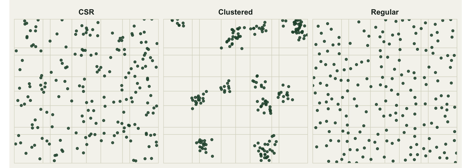
Counting in quadrats
The quadrat method turns the map into a table of counts. Lay a regular grid over the window, count how many points fall in each cell, and ask whether those counts look like they came from a Poisson process. Under CSR every quadrat has the same expected count, equal to the total number of points divided by the number of quadrats. Here a five by five grid gives 25 quadrats and an expected count of eight points each.
The signature of CSR is that the counts follow a Poisson distribution, for which the variance equals the mean. That gives us the variance-to-mean ratio (VMR). A ratio near one is consistent with randomness; a ratio above one means the counts are more variable than Poisson, the fingerprint of clustering; a ratio below one means the counts are unusually even, the fingerprint of regularity.
quadrat_stats <- function(p, Q = 5) {
  bx <- cut(p$x, breaks = seq(0, 1, length.out = Q + 1), include.lowest = TRUE)
  by <- cut(p$y, breaks = seq(0, 1, length.out = Q + 1), include.lowest = TRUE)
  counts <- as.vector(table(bx, by))     # all Q * Q cells, zeros included
  expected <- nrow(p) / (Q * Q)
  chi <- sum((counts - expected)^2 / expected)
  data.frame(
    n    = nrow(p),
    mean = mean(counts),
    var  = var(counts),
    vmr  = var(counts) / mean(counts),
    chisq = chi,
    df   = Q * Q - 1,
    p    = pchisq(chi, Q * Q - 1, lower.tail = FALSE)
  )
}

results <- bind_rows(
  CSR       = quadrat_stats(csr),
  Clustered = quadrat_stats(clustered),
  Regular   = quadrat_stats(regular),
  .id = "pattern"
)
results
pattern n mean var vmr chisq df p
1 CSR 200 8 8.083333 1.0104167 24.25 24 4.473784e-01
2 Clustered 200 8 114.833333 14.3541667 344.50 24 1.651389e-58
3 Regular 200 8 3.083333 0.3854167 9.25 24 9.970124e-01The numbers match the pictures. The random pattern has a variance of 8.08 against a mean of 8, so its VMR of 1.01 sits right on the CSR expectation. The clustered pattern has a variance of 114.8 and a VMR of 14.35: a handful of quadrats are packed while most are nearly empty. The regular pattern has a variance of only 3.08 and a VMR of 0.39, because inhibition keeps every quadrat close to the average.
From the ratio to a test
The variance-to-mean ratio also gives a formal test, because Pearson’s quadrat statistic is nothing more than the ratio in disguise. With equal expected counts, the chi-squared statistic equals the number of quadrats minus one, multiplied by the VMR.
Q <- 5
data.frame(
  pattern = results$pattern,
  chisq        = results$chisq,
  vmr_identity = (Q * Q - 1) * results$vmr
)
pattern chisq vmr_identity
1 CSR 24.25 24.25
2 Clustered 344.50 344.50
3 Regular 9.25 9.25The two columns agree to the last decimal, which is a useful sanity check on any hand-rolled quadrat routine. Under CSR the statistic follows a chi-squared distribution with 24 degrees of freedom. The random pattern gives 24.25, almost exactly its expected value, and a p-value of 0.45, so we correctly fail to reject randomness. The clustered pattern gives 344.5, far into the upper tail, with a p-value near 1.7e-58. The regular pattern gives 9.25, which is smaller than the degrees of freedom rather than larger, so it lands in the lower tail with a p-value of 0.997: the counts are too even to be Poisson.
That last case is worth pausing on. A one-sided reading that only watches for large statistics would call the regular pattern “not significant” and stop. The full picture needs both tails, because clustering inflates the statistic while regularity deflates it, and both are departures from CSR.
What quadrats can and cannot see
The quadrat test is coarse by design, and the coarseness is a choice you make when you pick the grid. Too few quadrats and the test has little power to detect anything; too many and the expected counts drop below about five per cell, at which point the chi-squared approximation starts to fail. The five by five grid used here keeps the expected count at eight, comfortably above that floor.
The deeper limitation is that quadrats only see structure at the scale of the cell. They register whether density varies from cell to cell, but they cannot tell you at what distance points attract or repel one another, and they throw away the exact coordinates you worked to collect. A pattern that is clustered at a scale much smaller than the quadrat can pass the test unnoticed, because the clumps hide inside single cells.
That is the motivation for everything that follows. The next post keeps the exact coordinates and measures the distance from each point to its nearest neighbour, which recovers the fine-scale information the grid discards. From there the series builds up to functions that describe the pattern across a whole range of distances at once.
References
Clark, P.J. and Evans, F.C. (1954) Ecology 35(4): 445-453. doi:10.2307/1931034
Ripley, B.D. (1977) Journal of the Royal Statistical Society Series B 39(2): 172-192. doi:10.1111/j.2517-6161.1977.tb01615.x
Wiegand, T. and Moloney, K.A. (2014) Handbook of Spatial Point-Pattern Analysis in Ecology. Chapman and Hall/CRC. ISBN 978-1-4200-8254-8
Diggle, P.J. (2013) Statistical Analysis of Spatial and Spatio-Temporal Point Patterns, 3rd edition. Chapman and Hall/CRC. ISBN 978-1-4665-6023-9