library(rgbif)

key <- name_backbone("Pulsatilla patens")$usageKey
raw <- occ_search(taxonKey = key, hasCoordinate = TRUE, limit = 2000)$data

# iNaturalist records directly, through the spocc package:
# spocc::occ(query = "Pulsatilla patens", from = "inat", limit = 2000)Cleaning GBIF and iNaturalist records in R
R
sf
data cleaning
GBIF
ecology tutorial
Occurrence records from GBIF and iNaturalist need cleaning. In R: drop impossible and duplicate coordinates, flag low precision, and map the result with sf.
Step 33 of the Tidy Ecology course, Part seven: put it on a map.
Updated 27 September 2026: a new section, What a centroid does to a niche, measures how records moved to a country centroid widen or narrow a fitted niche, and how far collapsing identical coordinates undoes it.
Every richness map and every species distribution model starts from the same raw material: a table of where a species has been recorded. The large aggregators, GBIF and iNaturalist, put millions of those records within reach of a single function call. They also hand you records sitting at zero degrees latitude and longitude, records pinned to a country centroid, museum specimens with the collector’s home town as the coordinate, and the same observation entered three times. None of that is unusual, and none of it is the aggregator’s fault: the data is a merge of thousands of sources. The work is yours, before any analysis is trustworthy. This post walks the cleaning that turns a raw pull into a defensible set of points.
Getting the records
The rgbif package is the R client for the GBIF API. For a single species you look up its backbone key, then request georeferenced records. iNaturalist research-grade observations flow into GBIF as well, so the same pull reaches them; for iNaturalist directly, spocc wraps its API. The call below is shown but not run, because a live pull is a moving target: the database changes daily and the API rate-limits, so nothing here would reproduce.
For a large or repeatable download use occ_download() rather than occ_search(): it queues a full extract server-side and returns a citable DOI, which the GBIF data-use terms ask you to keep. What follows works from a small saved extract bundled with this post, with the same columns occ_search() returns. The coordinates are illustrative, not a real locality.
library(dplyr)
library(sf)
library(ggplot2)

paper <- "#f5f4ee"; ink <- "#16241d"; forest <- "#275139"
gold  <- "#cda23f"; abandoned <- "#b5534e"; faint <- "#5d6b61"; line <- "#dad9ca"

theme_te <- theme_minimal(base_size = 12) +
  theme(panel.grid.minor = element_blank(),
        panel.grid.major = element_line(colour = line, linewidth = 0.3),
        plot.background = element_rect(fill = paper, colour = NA),
        panel.background = element_rect(fill = paper, colour = NA),
        axis.title = element_text(colour = ink),
        axis.text = element_text(colour = faint),
        plot.title = element_text(colour = ink, face = "bold"))
records <- read.csv("occurrences_raw.csv", stringsAsFactors = FALSE,
na.strings = "")
nrow(records)[1] 43Forty-three records, with the fields GBIF returns: a species name, decimal latitude and longitude, a coordinate uncertainty in metres, the basis of record, a year, an occurrence status, and a country code.
head(records[, c("decimalLatitude", "decimalLongitude",
                 "coordinateUncertaintyInMeters", "basisOfRecord",
                 "occurrenceStatus")], 4)
decimalLatitude decimalLongitude coordinateUncertaintyInMeters
1 47.09602 26.46606 1000
2 46.66959 22.05218 1000
3 45.42042 25.38712 250
4 45.85717 21.09694 1000
basisOfRecord occurrenceStatus
1 PRESERVED_SPECIMEN PRESENT
2 HUMAN_OBSERVATION PRESENT
3 HUMAN_OBSERVATION <NA>
4 OBSERVATION <NA>The problems hiding in this table are the common ones: rows with no coordinate at all, a row at exactly zero latitude and longitude (the “null island” off West Africa where missing values often land), an impossible latitude, coordinates so imprecise they could be anywhere in a county, exact duplicates, an absence dressed as a record, and a fossil that has no place in a present-day distribution. Each cleaning step below targets one of these, and reports how many rows are left.
Coordinates that could be real
The first pass keeps only rows whose coordinates exist and fall inside the possible range. Latitude runs from -90 to 90 and longitude from -180 to 180; anything outside is a data-entry error. The zero-zero point is dropped explicitly, because it is almost always a missing value that was silently coerced rather than a genuine record in the Gulf of Guinea.
clean <- records |>
  filter(!is.na(decimalLatitude), !is.na(decimalLongitude)) |>
  filter(decimalLatitude != 0 | decimalLongitude != 0) |>
  filter(between(decimalLatitude, -90, 90),
         between(decimalLongitude, -180, 180))
nrow(clean)
[1] 39That removes four rows: the two with a missing coordinate, the null-island point, and the impossible latitude. Thirty-nine remain.
Presence, and living records
An occurrence table can carry absences and fossils, and neither belongs in a map of where a species currently grows. GBIF marks absences with occurrenceStatus, and records the kind of evidence in basisOfRecord. Here we keep presences (or rows that leave the field blank) and observation or specimen records, which drops the fossil.
clean <- clean |>
  filter(is.na(occurrenceStatus) | occurrenceStatus == "PRESENT") |>
  filter(basisOfRecord %in% c("HUMAN_OBSERVATION", "PRESERVED_SPECIMEN",
                              "MACHINE_OBSERVATION", "OBSERVATION"))
nrow(clean)
[1] 37Two more gone, the flagged absence and the fossil specimen, leaving thirty-seven.
Precision you can use
A coordinate carries a stated uncertainty. A record good to 100 metres and one good to 50 kilometres are not the same evidence, and mixing them quietly degrades any analysis at a fine grain. The right ceiling depends on the question; for a two-kilometre richness grid, ten kilometres is already generous. Rows with no stated uncertainty are kept here rather than discarded, since a blank is common and not the same as a bad value, but that is a judgement worth stating out loud.
clean <- clean |>
  filter(is.na(coordinateUncertaintyInMeters) |
         coordinateUncertaintyInMeters <= 10000)
nrow(clean)
[1] 35The two coordinates uncertain to fifty kilometres drop out. Thirty-five left.
The same record, twice
Merged databases duplicate. The same observation can arrive from the original recorder and again through an aggregating dataset, identical in species and position. Collapsing on the fields that define a duplicate removes the copies while keeping the first of each.
clean <- clean |>
  distinct(species, decimalLatitude, decimalLongitude, .keep_all = TRUE)
nrow(clean)
[1] 32Three duplicate rows go, and thirty-two remain.
Inside the study region
The last step is spatial, so the records become an sf object. Turning the two coordinate columns into geometry with st_as_sf() lets the points be tested against a polygon: here a bounding box around the region of interest, which discards the two stray points that sit far to the west, one of them out in the Atlantic.
pts <- st_as_sf(clean, coords = c("decimalLongitude", "decimalLatitude"),
                crs = 4326, remove = FALSE)

region <- st_as_sfc(st_bbox(c(xmin = 20, ymin = 44, xmax = 28, ymax = 49),
                            crs = st_crs(4326)))
inside <- st_within(pts, region, sparse = FALSE)[, 1]
pts    <- pts[inside, ]
nrow(pts)
[1] 30Thirty points survive from the forty-three we started with. Thirteen removals, none of them arbitrary: each answered a specific, statable objection to a record.
ggplot() +
  geom_sf(data = region, fill = NA, colour = faint, linewidth = 0.4) +
  geom_sf(data = pts, colour = forest, size = 2.4, alpha = 0.9) +
  labs(x = NULL, y = NULL) +
  theme_te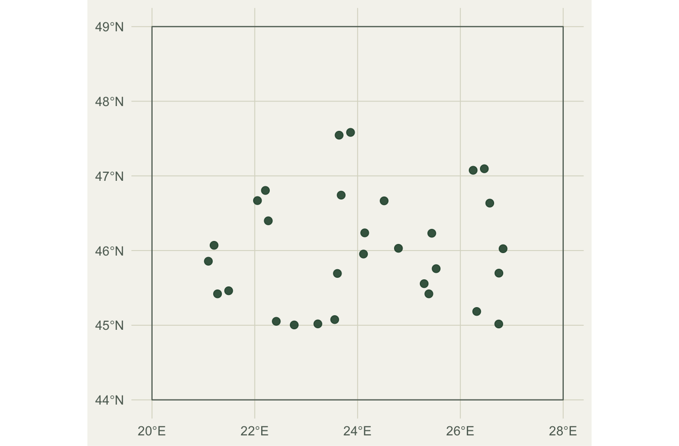
Doing this at scale
Cleaning by hand is worth doing once, to see what each rule removes. For many species or millions of records, the CoordinateCleaner package packages the same logic and adds tests that are awkward to write yourself: flagging points on country and province centroids, points at the GBIF headquarters or at biodiversity institutions, and points in the sea, all against built-in gazetteers.
library(CoordinateCleaner)

flags <- clean_coordinates(
  records,
  lon = "decimalLongitude", lat = "decimalLatitude", species = "species",
  tests = c("zeros", "equal", "duplicates", "seas", "centroids", "institutions"))

clean <- records[flags$.summary, ]   # keep records that passed every test
The manual pass and the package agree on the principle: a cleaning decision is only defensible if you can say which problem it fixes.
What a centroid does to a niche
A specimen label that says only “Romania” can end up georeferenced to the middle of the country, and the record then sits on a country or province centroid. The climate at that point says nothing about where the plant grew. The "centroids" test above calls cc_cen() from CoordinateCleaner (Zizka et al. 2019), which flags records within a buffer (1 km by default in version 3.0.1) around the country and province centroids in the package’s gazetteer, the countryref table. What unflagged centroid records do to a species distribution model is known arithmetic, and the simulation below only reproduces it.
Take one environmental gradient with flat availability from -4 to 4, and records that follow a Gaussian response with optimum 0 and tolerance 0.8 (the standard deviation of the curve). Replace a share e of the 400 records by copies of one centroid value d. On a flat gradient the log-quadratic presence-background fit (the point-process model that MaxEnt as a Poisson point process shows MaxEnt and weighted logistic regression to be) is a normal curve whose mean and variance, inside the window, equal those of the records. The records are now a mixture, so the optimum moves to e * d and the tolerance becomes the mixture’s standard deviation, sqrt((1 - e) * tol^2 + e * (1 - e) * d^2), which ignores the window edge. It exceeds tol only when the centroid is more than tol / sqrt(1 - e) from the optimum; a nearer centroid narrows the niche. The shares, the three centroid positions and the 100 data sets per cell were fixed before running.
cen_avail <- seq(-4, 4, length.out = 2001)   # flat availability: quadrature nodes
fit_niche <- function(x_rec) {                # log-quadratic point process by optim
  nll <- function(b) { eta <- b[1] * cen_avail + b[2] * cen_avail^2; top <- max(eta)
    -(sum(b[1] * x_rec + b[2] * x_rec^2) -
        length(x_rec) * (top + log(mean(exp(eta - top))))) }
  b <- optim(c(0, -1), nll, method = "BFGS")$par
  c(opt = -b[1] / (2 * b[2]), tol = sqrt(-1 / (2 * b[2])))
}
tol_true <- 0.8; n_rec <- 400; n_cen_rep <- 100
mix_tol <- function(e, d) sqrt((1 - e) * tol_true^2 + e * (1 - e) * d^2)  # the formula
cen_design <- expand.grid(share = c(0.02, 0.05, 0.10), cen = c(0, 1.5, 3))
set.seed(348)
cen_fits <- t(sapply(seq_len(nrow(cen_design)), function(i) {
  e <- cen_design$share[i]; d <- cen_design$cen[i]
  fits <- replicate(n_cen_rep, {
    x_rec <- rnorm(n_rec, 0, tol_true); x_rec <- x_rec[abs(x_rec) < 4]
    k <- round(e * length(x_rec))                # records moved to the centroid
    x_bad <- c(x_rec[seq_len(length(x_rec) - k)], rep(d, k))
    c(fit_niche(x_bad), sd_rec = sqrt(mean((x_bad - mean(x_bad))^2)),  # records' own SD
      thin = fit_niche(unique(x_bad)))
  })
  c(rowMeans(fits), se_tol = sd(fits["tol", ]) / sqrt(n_cen_rep))
}))
cen_tab <- data.frame(cen_design, cen_fits,
                      cf_tol = mix_tol(cen_design$share, cen_design$cen),
                      cf_opt = cen_design$share * cen_design$cen)
round(cen_tab, 3)
share cen opt tol sd_rec thin.opt thin.tol se_tol cf_tol cf_opt
1 0.02 0.0 -0.005 0.796 0.796 -0.005 0.803 0.002 0.792 0.000
2 0.05 0.0 -0.004 0.778 0.778 -0.004 0.797 0.003 0.780 0.000
3 0.10 0.0 0.000 0.761 0.761 0.000 0.801 0.003 0.759 0.000
4 0.02 1.5 0.031 0.816 0.816 0.005 0.799 0.003 0.819 0.030
5 0.05 1.5 0.073 0.841 0.841 0.002 0.798 0.003 0.846 0.075
6 0.10 1.5 0.156 0.877 0.877 0.011 0.797 0.003 0.882 0.150
7 0.02 3.0 0.051 0.892 0.892 -0.001 0.807 0.002 0.896 0.060
8 0.05 3.0 0.147 1.019 1.018 0.005 0.814 0.002 1.018 0.150
9 0.10 3.0 0.305 1.186 1.179 0.010 0.818 0.002 1.177 0.300cen_row <- function(e, d) cen_tab[cen_tab$share == e & cen_tab$cen == d, ]
cen_edge <- cen_tab$share == 0.10 & cen_tab$cen == 3 # the widest curve
stopifnot(which.max(abs(cen_tab$tol - cen_tab$cf_tol)) == which(cen_edge))In every cell the fitted tolerance is within 0.009 of the formula (Monte Carlo standard error of each mean at most 0.003); the largest gap, ten per cent at a centroid of 3, is the window edge. There the fit sits 0.007 above the records’ own standard deviation (sd_rec), against at most 0.001 in the other cells, because the curve has to be a little wider than the records for its part inside -4 to 4 to match them. Five per cent of the records on a centroid 3.75 tolerances from the optimum take the fitted tolerance from 0.8 to 1.019 (formula 1.018) and move the optimum by 0.147; ten per cent give 1.186 and 0.305. The same ten per cent at the optimum narrow the curve to 0.761. Keeping one record per distinct value (unique(), which is what the distinct() step earlier in this post does to a pile of identical coordinates) puts every cell back between 0.797 and 0.818.
A pile of centroid records is one coordinate pair repeated many times, so counting pairs before the duplicate step is a cheap look for them.
coord_counts <- count(records, decimalLatitude, decimalLongitude, sort = TRUE)
head(coord_counts, 3)
decimalLatitude decimalLongitude n
1 46.66611 24.51669 2
2 46.74242 23.68098 2
3 47.09602 26.46606 2records[records$countryCode %in% "PT",
c("decimalLatitude", "decimalLongitude", "countryCode")] decimalLatitude decimalLongitude countryCode
38 39.5 -8 PTIn this post’s extract no pair occurs more than 2 times, and the 3 pairs seen twice are the copies the duplicate step removed. The extract does hold one centroid record: the row at 39.5, -8.0 (country code PT) sits exactly on one of the two Portugal country centroids in CoordinateCleaner’s countryref table (version 3.0.1), and it left with the region filter as one of the two stray points in the west. A single centroid record is not a pile, so only a gazetteer test such as cc_cen() finds it. Whether an unflagged centroid pile widens or narrows the niche depends on how far its environment lies from the species’ optimum in tolerances, which no coordinate test can see; the formula also assumes flat availability, which a real landscape rarely has. Collapsing to one record per coordinate merges genuine repeat visits to one site too, and centroids taken from two gazetteers that differ slightly escape an exact match.
Where to go next
The cleaned points are the input the rest of the spatial workflow assumes. Feeding them to a grid gives a species richness map; a continuous environmental surface calls for raster work with terra; and either feeds a species distribution model. The other half of cleaning is taxonomic: reconciling synonyms and misspelt names so that records for one species are actually counted together, which rgbif’s name_backbone() and the taxize package handle.
References
Chamberlain SA, Boettiger C 2017 PeerJ Preprints 5:e3304v1 (10.7287/peerj.preprints.3304v1)
Zizka A, Silvestro D, Andermann T, Azevedo J, Duarte Ritter C, Edler D, Farooq H, Herdean A, Ariza M, Scharn R, Svantesson S, Wengstrom N, Zizka V, Antonelli A 2019 Methods in Ecology and Evolution 10(5):744-751 (10.1111/2041-210X.13152)
Pebesma E 2018 The R Journal 10(1):439-446 (10.32614/RJ-2018-009)