---
title: "Integrated species distribution models in R"
description: "Combine presence-only records with a structured occupancy survey in one likelihood, correcting sampling bias and sharpening the environmental response."
date: "2026-05-23 12:00"
categories: [species distribution, data integration, point process, occupancy, ecology tutorial]
image: thumbnail.png
image-alt: "Point estimates of the environmental response slope with error bars from four estimators, ordered naive presence-only, presence-only plus effort, survey only and integrated, against a dashed horizontal line at the true response. The naive point sits highest with its bar clear of the dashed line, while the survey only bar is much the widest of the four."
---
Two kinds of data describe where a species lives, and they have opposite strengths. Opportunistic presence-only records are plentiful but sampled wherever people happen to go, so their density confounds the environment with survey effort. A structured survey visits chosen sites on a fixed protocol, so it is unbiased and carries an absolute scale, but it is expensive and therefore sparse. An integrated model fits both in a single likelihood, letting the structured survey calibrate the bias in the presence-only stream while the presence-only stream lends its coverage to the estimate.
This post builds that model from scratch in base R. We simulate one landscape with a known environmental response, sample it two ways, and compare four estimators: presence-only alone, presence-only with an effort covariate, the survey alone, and the integrated fit.
## A landscape and two samples
The intensity of a point process gives the expected number of individuals per unit area. We set a log-linear intensity driven by one environmental covariate, then thin the points by an accessibility surface that stands in for survey effort. Accessibility is correlated with the environment, which is what makes the naive presence-only estimate go wrong.
```{r setup}
#| code-fold: true
#| code-summary: "Setup: packages, colours and plot theme"
#| results: hide
#| message: false
#| warning: false
knitr::opts_chunk$set(echo = TRUE, message = FALSE, warning = FALSE,
                      fig.width = 7.5, fig.height = 4.6, dpi = 150, dev = "png")
library(ggplot2)
te <- list(ink="#16241d", body="#2c3a31", forest="#275139", label="#46604a",
           sage="#93a87f", paper="#f5f4ee", line="#dad9ca", card="#ffffff",
           faint="#5d6b61", grazed="#cda23f", mown="#2f8f63", abandoned="#b5534e",
           grad_low="#c9b458", grad_high="#1d5b4e")
theme_te <- function(base_size = 12) {
  theme_minimal(base_size = base_size) +
    theme(text=element_text(colour=te$body),
          plot.title=element_text(colour=te$ink, face="bold", size=base_size+1),
          plot.subtitle=element_text(colour=te$faint, size=base_size-1),
          axis.title=element_text(colour=te$label),
          axis.text=element_text(colour=te$faint, size=base_size-2),
          panel.grid.major=element_line(colour=te$line, linewidth=0.3),
          panel.grid.minor=element_blank(),
          panel.background=element_rect(fill=te$paper, colour=NA),
          plot.background=element_rect(fill=te$paper, colour=NA),
          legend.title=element_text(colour=te$label, size=base_size-2),
          legend.text=element_text(colour=te$faint, size=base_size-2),
          strip.text=element_text(colour=te$ink, face="bold", size=base_size-1),
          strip.background=element_rect(fill=te$paper, colour=NA),
          plot.margin=margin(10,12,10,10))
}
```
```{r smooth-field}
# a smooth spatial field on a g x g grid, standardised
smooth_field <- function(g, l, seed) {
  set.seed(seed)
  u <- (seq_len(g) - 0.5) / g
  D <- outer(u, u, function(a, b) exp(-(a - b)^2 / (2 * l^2)))
  Sm <- D / rowSums(D)
  as.numeric(scale(as.numeric(Sm %*% matrix(rnorm(g * g), g, g) %*% t(Sm))))
}

g     <- 50                 # grid resolution
Acell <- 1 / (g * g)        # area of one grid cell (unit square)
x     <- smooth_field(g, 0.18, 4711)                 # environmental covariate
raw   <- smooth_field(g, 0.18, 9001)
acc   <- as.numeric(scale(0.6 * x + sqrt(1 - 0.36) * raw))  # accessibility, rho ~ 0.6

b1_true <- 1.0              # true environmental response
a1_true <- 1.6             # effort effect on detection of records
p_true  <- 0.40            # per-visit detection in the survey
Asite   <- 0.0004          # area of one survey site
EN      <- 4000            # expected number of individuals
b0_true <- log(EN / (Acell * sum(exp(b1_true * x))))
round(c(cor_x_acc = cor(x, acc), b0_true = b0_true), 3)
```
```{r simulate}
set.seed(1)
lambda <- exp(b0_true + b1_true * x)                 # true intensity surface
N      <- rpois(1, Acell * sum(lambda))
cell   <- sample(length(x), N, replace = TRUE, prob = lambda / sum(lambda))
bias   <- exp(a1_true * acc)                          # effort-driven thinning
keep   <- rbinom(N, 1, pmin(1, bias[cell] / max(bias)))
po     <- tabulate(cell[keep == 1], nbins = length(x))  # presence-only counts per cell

nsite  <- 300
ssite  <- sample(length(x), nsite)                    # structured survey sites
K      <- 4                                            # repeat visits
psi    <- 1 - exp(-Asite * exp(b0_true + b1_true * x[ssite]))  # cloglog occupancy
z      <- rbinom(nsite, 1, psi)
y      <- rbinom(nsite, K, z * p_true)
c(records = sum(po), sites_detected = sum(y > 0), true_occupancy = round(mean(psi), 3))
```
The complementary log-log link is the glue here. If individuals fall as a Poisson process of intensity lambda, the probability that a site of area A holds at least one individual is 1 minus exp(-A times lambda), which is exactly a cloglog occupancy model with an offset of log(A). That shared form lets the survey and the point process speak about the same intensity surface.
## Four estimators
We fit each model by maximising its likelihood with `optim`. The presence-only likelihood is the standard inhomogeneous Poisson process likelihood evaluated on the grid; the occupancy likelihood marginalises over the latent presence state.
```{r fits}
# presence-only point process likelihood on the grid
nll_po <- function(par, use_acc) {
  b1 <- par[1]; s0 <- par[2]
  lp <- s0 + b1 * x
  if (use_acc) lp <- lp + par[3] * acc
  mu <- exp(lp)
  -(sum(po * log(mu)) - Acell * sum(mu))
}
fit_po_naive  <- optim(c(1, 0),    nll_po, use_acc = FALSE, method = "BFGS", hessian = TRUE)
fit_po_effort <- optim(c(1, 0, 0), nll_po, use_acc = TRUE,  method = "BFGS", hessian = TRUE)

# survey-only occupancy, marginalising the latent state
nll_occ <- function(par) {
  b0 <- par[1]; b1 <- par[2]; p <- plogis(par[3])
  ps <- 1 - exp(-Asite * exp(b0 + b1 * x[ssite]))
  -sum(log(ps * dbinom(y, K, p) + (1 - ps) * (y == 0)))
}
fit_occ <- optim(c(b0_true, 1, 0), nll_occ, method = "BFGS", hessian = TRUE)

# integrated: shared b0, b1; the records add their own intercept and effort slope
nll_joint <- function(par) {
  b0 <- par[1]; b1 <- par[2]; a0 <- par[3]; p <- plogis(par[4]); a1 <- par[5]
  mu <- exp(b0 + b1 * x + a0 + a1 * acc)
  ll_po  <- sum(po * log(mu)) - Acell * sum(mu)
  ps     <- 1 - exp(-Asite * exp(b0 + b1 * x[ssite]))
  ll_occ <- sum(log(ps * dbinom(y, K, p) + (1 - ps) * (y == 0)))
  -(ll_po + ll_occ)
}
fit_joint <- optim(c(b0_true, 1, -3, 0, 0), nll_joint, method = "BFGS", hessian = TRUE)

se <- function(f, i) sqrt(diag(solve(f$hessian)))[i]
b1_naive  <- fit_po_naive$par[1]
b1_effort <- fit_po_effort$par[1]
b1_occ    <- fit_occ$par[2];   se_occ   <- se(fit_occ, 2)
b1_joint  <- fit_joint$par[2]; se_joint <- se(fit_joint, 2)
round(c(naive = b1_naive, effort = b1_effort, occupancy = b1_occ, integrated = b1_joint), 3)
```
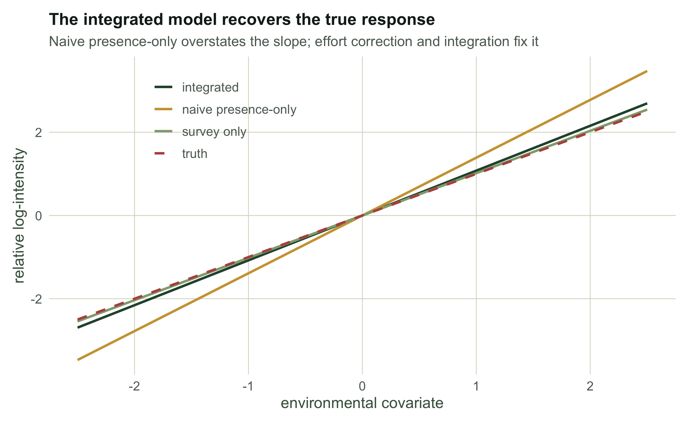
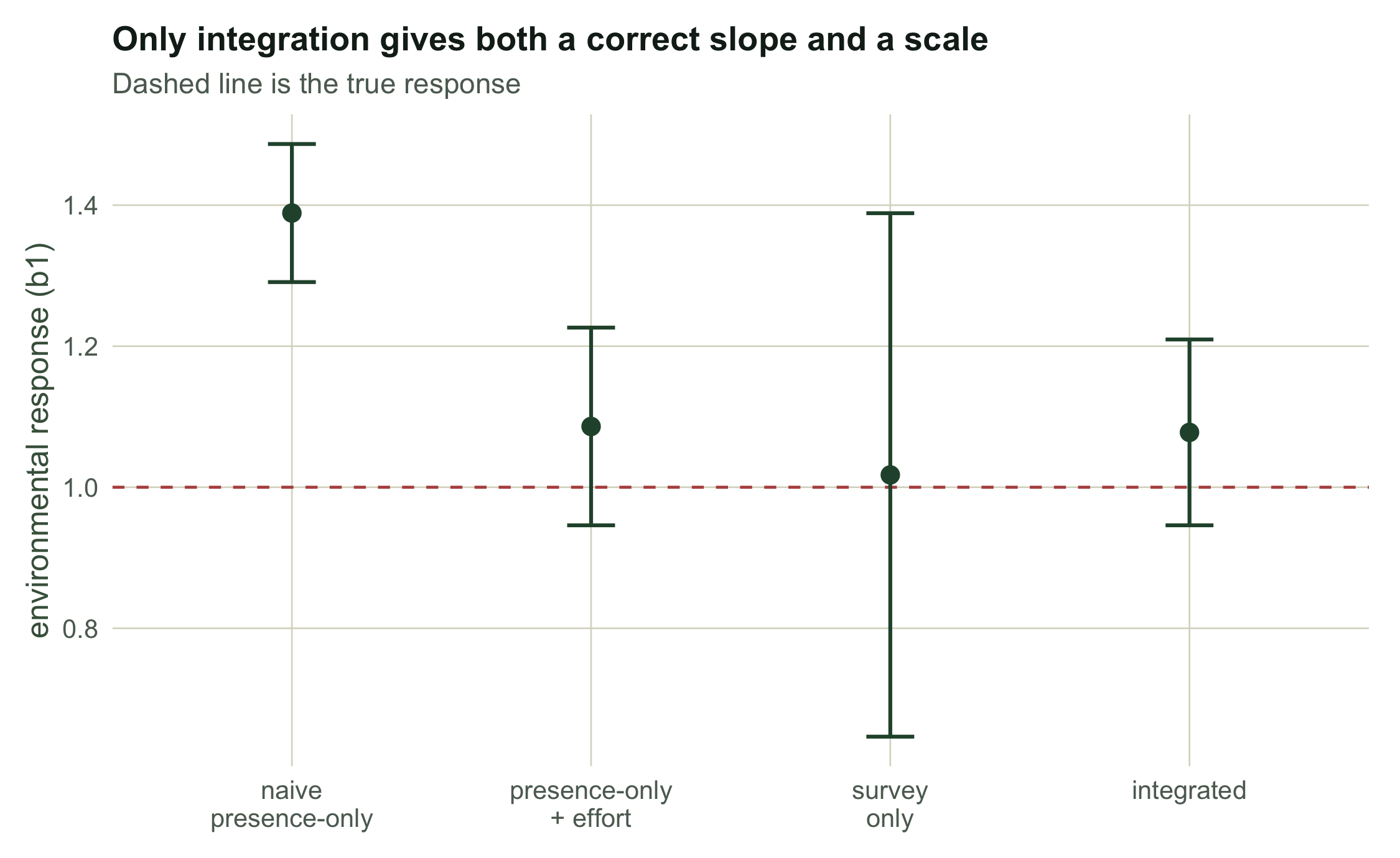
The naive presence-only slope is `r round(b1_naive, 2)` against a truth of `r b1_true`. Accessibility is missing from that fit, so the slope carries the effort surface as well as the environment and is not an estimate of the environmental response. Add the effort covariate and the point process returns `r round(b1_effort, 2)`, but its intercept mixes the true abundance with the sampling rate, so it has no absolute scale. The survey alone gives `r round(b1_occ, 2)` and does carry a scale, with a standard error of `r round(se_occ, 3)`. The integrated fit puts the slope at `r round(b1_joint, 2)` while cutting the standard error to `r round(se_joint, 3)`, about `r round(100 * se_joint / se_occ)` per cent of the survey-only value.
```{r}
#| label: fig-response
#| fig-cap: "Relative log-intensity against the environmental covariate for three of the four estimators, with the truth dashed."
#| fig-alt: "Line plot of relative log-intensity against the environmental covariate. Four straight lines cross near the centre of the x range: a dashed line for the truth and solid lines for the naive presence-only, survey-only and integrated fits, each drawn at its own slope."
xg <- seq(-2.5, 2.5, length.out = 100)
rel <- function(b1) b1 * xg - b1 * mean(xg)
dl <- rbind(
  data.frame(x = xg, y = rel(b1_true),  who = "truth"),
  data.frame(x = xg, y = rel(b1_naive), who = "naive presence-only"),
  data.frame(x = xg, y = rel(b1_occ),   who = "survey only"),
  data.frame(x = xg, y = rel(b1_joint), who = "integrated"))
ggplot(dl, aes(x, y, colour = who, linetype = who)) +
  geom_line(linewidth = 0.9) +
  scale_colour_manual(values = c("truth" = te$abandoned, "naive presence-only" = te$grazed,
                                 "survey only" = te$sage, "integrated" = te$forest)) +
  scale_linetype_manual(values = c("truth" = "dashed", "naive presence-only" = "solid",
                                   "survey only" = "solid", "integrated" = "solid")) +
  labs(x = "environmental covariate", y = "relative log-intensity",
       title = "Fitted relative log-intensity: naive, survey only and integrated",
       subtitle = "Each solid line is drawn at its estimator's fitted slope; the dashed line is the truth",
       colour = NULL, linetype = NULL) +
  theme_te() + theme(legend.position = "inside", legend.position.inside = c(0.28, 0.8))
```
## Does it hold up across data sets?
One realisation could be luck. We repeat the whole exercise many times and record the slope from the survey-only and integrated fits.
```{r mc}
run_one <- function(seed) {
  set.seed(seed)
  lam  <- exp(b0_true + b1_true * x)
  Nn   <- rpois(1, Acell * sum(lam))
  cl   <- sample(length(x), Nn, replace = TRUE, prob = lam / sum(lam))
  bi   <- exp(a1_true * acc)
  kp   <- rbinom(Nn, 1, pmin(1, bi[cl] / max(bi)))
  po2  <- tabulate(cl[kp == 1], nbins = length(x))
  ss   <- sample(length(x), nsite)
  ps   <- 1 - exp(-Asite * exp(b0_true + b1_true * x[ss]))
  zz   <- rbinom(nsite, 1, ps); yy <- rbinom(nsite, K, zz * p_true)
  nll_o <- function(par) { b0<-par[1];b1<-par[2];p<-plogis(par[3])
    q<-1-exp(-Asite*exp(b0+b1*x[ss])); -sum(log(q*dbinom(yy,K,p)+(1-q)*(yy==0))) }
  nll_j <- function(par) { b0<-par[1];b1<-par[2];a0<-par[3];p<-plogis(par[4]);a1<-par[5]
    mu<-exp(b0+b1*x+a0+a1*acc); lpo<-sum(po2*log(mu))-Acell*sum(mu)
    q<-1-exp(-Asite*exp(b0+b1*x[ss])); lo<-sum(log(q*dbinom(yy,K,p)+(1-q)*(yy==0))); -(lpo+lo) }
  fo <- tryCatch(optim(c(b0_true,1,0), nll_o, method="BFGS", hessian=TRUE), error=function(e) NULL)
  fj <- tryCatch(optim(c(b0_true,1,-3,0,0), nll_j, method="BFGS", hessian=TRUE), error=function(e) NULL)
  if (is.null(fo) || is.null(fj)) return(rep(NA, 4))
  so <- sqrt(diag(solve(fo$hessian)))[2]; sj <- sqrt(diag(solve(fj$hessian)))[2]
  c(fo$par[2], so, fj$par[2], sj)
}
M  <- 100
mc <- t(sapply(1:M, function(m) run_one(1000 + m)))
mc <- mc[stats::complete.cases(mc), ]
cover <- function(est, s) mean(abs(est - b1_true) <= 1.96 * s)
occ_sd <- sd(mc[, 1]); joint_sd <- sd(mc[, 3])
round(c(occ_mean = mean(mc[, 1]), joint_mean = mean(mc[, 3]),
        occ_sd = occ_sd, joint_sd = joint_sd,
        sd_ratio = joint_sd / occ_sd,
        joint_coverage = cover(mc[, 3], mc[, 4])), 3)
```
Across `r nrow(mc)` data sets both estimators centre near `r b1_true`, but the integrated slope varies less: its standard deviation is about `r round(100 * joint_sd / occ_sd)` per cent of the survey-only spread. That is the whole point of integration. You are not choosing between the two data sets; you are letting each cover the other's weakness. Two things to keep in mind when reading these figures. The `r round(100 * se_joint / se_occ)` per cent quoted earlier came from one fit and one pair of standard errors, so it is a draw from this same distribution rather than the rule. And the joint interval covers the truth in `r round(cover(mc[, 3], mc[, 4]), 3)` of these data sets, against a nominal 0.95. A single fit cannot tell you whether its model-based standard error is the right width; a sweep like this one can.
```{r}
#| label: fig-forest
#| fig-cap: "Slope estimates with 95 per cent intervals from four estimators, against a dashed line at the truth."
#| fig-alt: "Point estimates with error bars for the slope from four estimators, ordered left to right as naive presence-only, presence-only with effort, survey only and integrated, plotted on an environmental response axis against a dashed horizontal line at the true value. The bars differ in width, and the four points do not sit at the same height: three lie close together near the dashed line and one sits further from it."
est <- data.frame(
  method = factor(c("naive\npresence-only", "presence-only\n+ effort", "survey\nonly", "integrated"),
                  levels = c("naive\npresence-only", "presence-only\n+ effort", "survey\nonly", "integrated")),
  b1 = c(b1_naive, b1_effort, b1_occ, b1_joint),
  se = c(se(fit_po_naive, 1), se(fit_po_effort, 1), se_occ, se_joint))
p_forest <- ggplot(est, aes(method, b1)) +
  geom_hline(yintercept = b1_true, colour = te$abandoned, linetype = "dashed") +
  geom_errorbar(aes(ymin = b1 - 1.96 * se, ymax = b1 + 1.96 * se), width = 0.16,
                colour = te$forest, linewidth = 0.7) +
  geom_point(size = 2.8, colour = te$forest) +
  labs(x = NULL, y = "environmental response (b1)",
       title = "Slope and 95 per cent interval from each estimator",
       subtitle = "Dashed line is the true response") +
  theme_te()
p_forest
```
```{r}
#| label: thumb
#| include: false
thumb_title <- paste(strwrap("Slope and interval from four estimators", 46),
collapse = "\n")
ggsave("thumbnail.png",
p_forest + labs(title = thumb_title) +
theme(plot.title = element_text(size = 13, face = "bold"),
plot.subtitle = element_text(size = 9.5),
plot.margin = margin(8, 14, 8, 8)),
width = 7.5, height = 5.4, dpi = 100, bg = te$paper)
```
## When to reach for this
Integration earns its keep when a large biased data set sits beside a small clean one, and when a plausible covariate explains the bias. It cannot rescue you if the bias is unmodelled and correlated with the environment, and it assumes both streams see the same underlying surface. The next tutorial checks exactly that assumption, showing how a joint model can hide a disagreement between its two data sources.
## References
Dorazio RM 2014 Global Ecology and Biogeography 23(12):1472-1484 (10.1111/geb.12216)
Fithian W, Elith J, Hastie T, Keith DA 2015 Methods in Ecology and Evolution 6(4):424-438 (10.1111/2041-210X.12242)
Koshkina V, Wang Y, Gordon A, Dorazio RM, White M, Stone L 2017 Methods in Ecology and Evolution 8(4):420-430 (10.1111/2041-210X.12738)
Fletcher RJ, Hefley TJ, Robertson EP, Zuckerberg B, McCleery RA, Dorazio RM 2019 Ecology 100(6):e02710 (10.1002/ecy.2710)
Miller DAW, Pacifici K, Sanderlin JS, Reich BJ 2019 Methods in Ecology and Evolution 10(1):22-37 (10.1111/2041-210X.13110)
Isaac NJB, Jarzyna MA, Keil P, et al. 2020 Trends in Ecology and Evolution 35(1):56-67 (10.1016/j.tree.2019.08.006)
## Related tutorials
- [Logistic regression for presence-absence](../logistic-regression-presence-absence/)
- [MaxEnt as a Poisson point process](../maxent-as-a-point-process/)
- [Cleaning GBIF occurrence data](../cleaning-gbif-occurrence-data/)
- [Checking an integrated SDM](../checking-an-integrated-sdm/)