---
title: "Checking an integrated SDM"
description: "A joint model can hide a conflict between its two data sources. Ordinary goodness of fit is fooled, but a source-conflict check tests whether they agree."
date: "2026-05-23 15:00"
categories: [data integration, model checking, species distribution, goodness of fit, ecology tutorial]
image: thumbnail.png
image-alt: "A single panel of three bars, labelled survey only, presence-only and joint along the horizontal axis, against a vertical axis of the environmental response b1 running from 0.0 to 1.5, with a dashed horizontal line across the panel at the true slope of 1.0."
---
An integrated species distribution model borrows strength from two data sets at once, and that is its appeal. It is also its blind spot. When the two sources disagree about the thing they share, the joint fit still returns a single shared estimate, and in the fits below that estimate lands between the two single-source values. Worse, the usual fit diagnostics look clean, because each stream on its own is fit adequately. The disagreement lives in the space between them.
This is the closing post of the integrated-model thread. It builds a case where a joint model is misled by a bad assumption, shows that an ordinary goodness-of-fit check waves it through, and then builds a targeted check that catches it. If you have not seen the model itself, start with [integrated species distribution models](../integrated-species-distribution-model/).
## Two sources that can disagree
We reuse the setup from the previous post: presence-only records whose density is biased by accessibility, plus a structured survey that is unbiased. Both speak about one environmental response. The catch is that accessibility is correlated with the environment, so if we model the presence-only bias wrongly, the accessibility signal has no route into the records likelihood except through the shared environmental response, while the survey estimate does not use the records at all.
```{r setup}
#| code-fold: true
#| code-summary: "Setup: packages, colours and plot theme"
#| results: hide
#| message: false
#| warning: false
knitr::opts_chunk$set(echo = TRUE, message = FALSE, warning = FALSE,
                      fig.width = 7.5, fig.height = 4.6, dpi = 150, dev = "png")
library(ggplot2)
te <- list(ink="#16241d", body="#2c3a31", forest="#275139", label="#46604a",
           sage="#93a87f", paper="#f5f4ee", line="#dad9ca", card="#ffffff",
           faint="#5d6b61", grazed="#cda23f", mown="#2f8f63", abandoned="#b5534e",
           grad_low="#c9b458", grad_high="#1d5b4e")
theme_te <- function(base_size = 12) {
  theme_minimal(base_size = base_size) +
    theme(text=element_text(colour=te$body),
          plot.title=element_text(colour=te$ink, face="bold", size=base_size+1),
          plot.subtitle=element_text(colour=te$faint, size=base_size-1),
          axis.title=element_text(colour=te$label),
          axis.text=element_text(colour=te$faint, size=base_size-2),
          panel.grid.major=element_line(colour=te$line, linewidth=0.3),
          panel.grid.minor=element_blank(),
          panel.background=element_rect(fill=te$paper, colour=NA),
          plot.background=element_rect(fill=te$paper, colour=NA),
          legend.title=element_text(colour=te$label, size=base_size-2),
          legend.text=element_text(colour=te$faint, size=base_size-2),
          strip.text=element_text(colour=te$ink, face="bold", size=base_size-1),
          strip.background=element_rect(fill=te$paper, colour=NA),
          plot.margin=margin(10,12,10,10))
}
```
```{r landscape}
smooth_field <- function(g, l, seed) {
  set.seed(seed)
  u <- (seq_len(g) - 0.5) / g
  D <- outer(u, u, function(a, b) exp(-(a - b)^2 / (2 * l^2)))
  Sm <- D / rowSums(D)
  as.numeric(scale(as.numeric(Sm %*% matrix(rnorm(g * g), g, g) %*% t(Sm))))
}

g <- 40; R <- g * g; Acell <- 1 / R
gx  <- smooth_field(g, 0.18, 4711)                       # environment
raw <- smooth_field(g, 0.18, 9001)
e   <- as.numeric(scale(resid(lm(raw ~ gx)))); rho <- 0.55
acc <- as.numeric(scale(rho * gx + sqrt(1 - rho^2) * e)) # accessibility, correlated with gx

b1_t <- 1.0; a0_t <- -0.5; a1_t <- 1.5; p_t <- 0.45
nsite <- 300; K <- 4; Asite <- Acell * 0.9; EN <- 1500
b0_t <- log(EN / (Acell * sum(exp(b1_t * gx))))
round(c(cor_x_acc = cor(gx, acc), b0 = b0_t), 3)
```
```{r simulate}
sim_one <- function(seed) {
  set.seed(seed)
  lam  <- exp(b0_t + b1_t * gx)
  N    <- rpois(1, Acell * sum(lam))
  cell <- sample(R, N, replace = TRUE, prob = lam / sum(lam))
  bias <- exp(a0_t + a1_t * acc)
  keep <- rbinom(N, 1, pmin(1, bias[cell] / max(bias)))
  po   <- tabulate(cell[keep == 1], nbins = R)             # presence-only counts
  ssite <- sample(R, nsite)
  psi  <- 1 - exp(-Asite * exp(b0_t + b1_t * gx[ssite]))
  z <- rbinom(nsite, 1, psi); y <- rbinom(nsite, K, z * p_t)
  list(po = po, y = y, ssite = ssite)
}
d <- sim_one(150); ssite <- d$ssite
c(records = sum(d$po), sites_detected = sum(d$y > 0), sites = nsite)
```
## Fitting three ways
We fit the shared environmental response three times: from the survey alone, from the records alone, and jointly. Each presence-only or joint fit carries a switch, `use_acc`, that decides whether the accessibility covariate is in the bias model. With it, the model is well specified. Without it, the accessibility bias is omitted, which is the mistake we want to catch.
```{r likelihoods}
nll_po <- function(par, po, use_acc) {
  b1 <- par[1]; s0 <- par[2]; lp <- s0 + b1 * gx
  if (use_acc) lp <- lp + par[3] * acc
  mu <- exp(lp); -(sum(po * log(mu)) - Acell * sum(mu))
}
fit_po <- function(po, use_acc)
  optim(if (use_acc) c(1, 0, 0) else c(1, 0), nll_po, po = po, use_acc = use_acc, method = "BFGS")

nll_su <- function(par, y) {
  b0 <- par[1]; b1 <- par[2]; p <- plogis(par[3])
  psi <- 1 - exp(-Asite * exp(b0 + b1 * gx[ssite]))
  -sum(log(psi * dbinom(y, K, p) + (1 - psi) * (y == 0)))
}
fit_su <- function(y) optim(c(b0_t, 1, 0), nll_su, y = y, method = "BFGS")

nll_jt <- function(par, po, y, use_acc) {
  b0 <- par[1]; b1 <- par[2]; a0 <- par[3]; p <- plogis(par[4])
  a1 <- if (use_acc) par[5] else 0
  mu <- exp(b0 + b1 * gx + a0 + a1 * acc)
  ll_po <- sum(po * log(mu)) - Acell * sum(mu)
  psi <- 1 - exp(-Asite * exp(b0 + b1 * gx[ssite]))
  ll_su <- sum(log(psi * dbinom(y, K, p) + (1 - psi) * (y == 0)))
  -(ll_po + ll_su)
}
fit_jt <- function(po, y, use_acc)
  optim(if (use_acc) c(b0_t, 1, a0_t, 0, 0) else c(b0_t, 1, a0_t, 0),
        nll_jt, po = po, y = y, use_acc = use_acc, method = "BFGS")
```
```{r scenarios}
su   <- fit_su(d$y); b1_su <- su$par[2]
po_w <- fit_po(d$po, TRUE);  jt_w <- fit_jt(d$po, d$y, TRUE)
po_m <- fit_po(d$po, FALSE); jt_m <- fit_jt(d$po, d$y, FALSE)
b1_po_w <- po_w$par[1]; b1_jt_w <- jt_w$par[2]; T_w <- b1_po_w - b1_su
b1_po_m <- po_m$par[1]; b1_jt_m <- jt_m$par[2]; T_m <- b1_po_m - b1_su
round(rbind(
  `well-specified` = c(survey = b1_su, presence_only = b1_po_w, joint = b1_jt_w, conflict_T = T_w),
  `misspecified`   = c(survey = b1_su, presence_only = b1_po_m, joint = b1_jt_m, conflict_T = T_m)), 3)
```
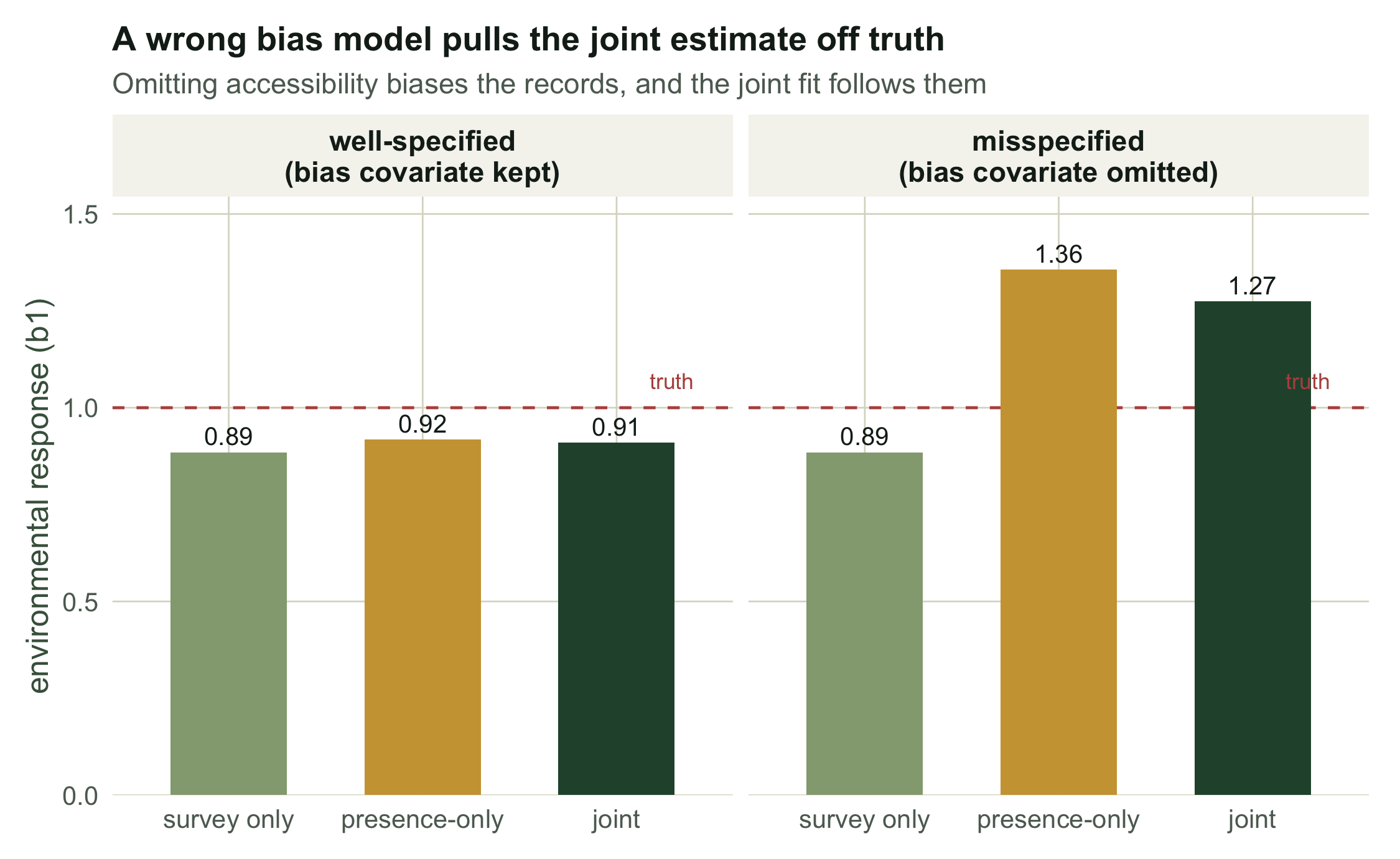
When the bias model is right, read the three estimates of the slope against the truth of `r b1_t`: the survey gives `r round(b1_su, 3)`, the records `r round(b1_po_w, 3)`, and the joint fit `r round(b1_jt_w, 3)`. The records and the survey differ by `r sprintf("%+.3f", T_w)`.
Omit accessibility and the picture changes. The survey is untouched at `r round(b1_su, 3)`, the records now read `r round(b1_po_m, 3)`, and the joint fit lands at `r round(b1_jt_m, 3)`. The records and the survey differ by `r sprintf("%+.3f", T_m)`.
```{r}
#| label: fig-sources
#| fig-cap: "The environmental slope by source under each scenario, with the true value marked by the dashed line and each bar labelled with its estimate."
#| fig-alt: "Grouped bars of the slope for survey, presence-only and joint in two panels; in the misspecified panel the presence-only and joint bars sit well above the dashed truth line."
d1 <- data.frame(
  scenario = rep(c("well-specified\n(bias covariate kept)", "misspecified\n(bias covariate omitted)"), each = 3),
  source = rep(c("survey only", "presence-only", "joint"), 2),
  b1 = c(b1_su, b1_po_w, b1_jt_w, b1_su, b1_po_m, b1_jt_m))
d1$scenario <- factor(d1$scenario, levels = unique(d1$scenario))
d1$source <- factor(d1$source, levels = c("survey only", "presence-only", "joint"))
ggplot(d1, aes(source, b1, fill = source)) +
  geom_col(width = 0.6) + facet_wrap(~scenario) +
  geom_hline(yintercept = b1_t, colour = te$abandoned, linetype = "dashed") +
  geom_text(aes(label = sprintf("%.2f", b1)), vjust = -0.4, size = 3.4, colour = te$ink) +
  annotate("text", x = 1.5, y = b1_t + 0.06, label = "truth", hjust = 0.5, size = 3, colour = te$abandoned) +
  scale_fill_manual(values = c("survey only" = te$sage, "presence-only" = te$grazed, "joint" = te$forest), guide = "none") +
  scale_y_continuous(limits = c(0, 1.5), expand = expansion(mult = c(0, 0.03))) +
  labs(x = NULL, y = "environmental response (b1)",
       title = "The environmental slope by source, under two bias models",
       subtitle = "Survey only, presence-only and joint in each panel, against the dashed true slope") +
  theme_te()
```
## Two goodness-of-fit checks
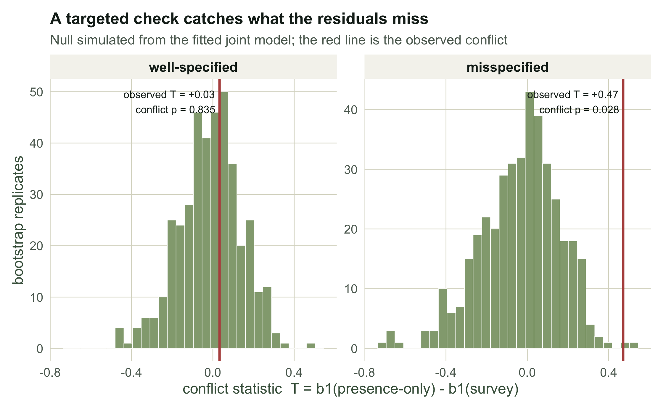
We compare two ways of asking whether the model fits, both calibrated by parametric bootstrap. The first is an ordinary omnibus check: a dispersion statistic for the presence-only counts against their fitted intensity. The second is targeted: the conflict statistic T, the gap between the environmental slope estimated from the records and from the survey. Under a correct joint model these two estimates agree, so T should sit near zero; a large T points straight at a disagreement the model cannot see.
```{r gof-helpers}
sim_from <- function(par, use_acc) {        # simulate both streams from a fitted joint model
  b0 <- par[1]; b1 <- par[2]; a0 <- par[3]; p <- plogis(par[4])
  a1 <- if (use_acc) par[5] else 0
  mu <- exp(b0 + b1 * gx + a0 + a1 * acc)
  po <- rpois(R, Acell * mu)
  psi <- 1 - exp(-Asite * exp(b0 + b1 * gx[ssite]))
  z <- rbinom(nsite, 1, psi); y <- rbinom(nsite, K, z * p)
  list(po = po, y = y)
}
po_pearson <- function(po, jtpar, use_acc) { # omnibus dispersion of the records
  b0 <- jtpar[1]; b1 <- jtpar[2]; a0 <- jtpar[3]
  a1 <- if (use_acc) jtpar[5] else 0
  mu <- exp(b0 + b1 * gx + a0 + a1 * acc) * Acell
  sum((po - mu)^2 / mu) / (R - length(jtpar))
}
boot_scen <- function(jt, use_acc, Tobs, Pobs, B) {
  Tstar <- numeric(B); Pstar <- numeric(B)
  for (b in 1:B) {
    sm <- sim_from(jt$par, use_acc)
    su2 <- fit_su(sm$y); po2 <- fit_po(sm$po, use_acc); jt2 <- fit_jt(sm$po, sm$y, use_acc)
    Tstar[b] <- po2$par[1] - su2$par[2]
    Pstar[b] <- po_pearson(sm$po, jt2$par, use_acc)
  }
  list(pT = mean(abs(Tstar) >= abs(Tobs)), pP = mean(Pstar >= Pobs), Tstar = Tstar)
}
```
```{r gof-run}
Pobs_w <- po_pearson(d$po, jt_w$par, TRUE)
Pobs_m <- po_pearson(d$po, jt_m$par, FALSE)
set.seed(2024); B <- 400
bw <- boot_scen(jt_w, TRUE,  T_w, Pobs_w, B)   # well-specified
bm <- boot_scen(jt_m, FALSE, T_m, Pobs_m, B)   # misspecified
round(rbind(
  `well-specified` = c(omnibus_p = bw$pP, conflict_p = bw$pT),
  `misspecified`   = c(omnibus_p = bm$pP, conflict_p = bm$pT)), 3)
```
The result is the point of the whole post. Under the wrong model the omnibus check gives a p-value of `r round(bm$pP, 3)`, not significant: the records sit close to the intensity surface the joint model fitted to them. Nothing to see. The targeted conflict check, on the same fit, returns `r round(bm$pT, 3)`. A small p here says the two sources do not agree about the slope they share, which is a question the omnibus statistic cannot ask. Under the correct model the same two checks return `r round(bw$pP, 3)` and `r round(bw$pT, 3)`.
```{r}
#| label: fig-conflict
#| fig-cap: "Bootstrap null distribution of the conflict statistic, one panel per scenario. The red line marks the observed conflict and the label beside it gives the bootstrap p-value."
#| fig-alt: "Two histograms of the bootstrapped conflict statistic; the observed value is central in the well-specified panel and far to the right in the misspecified panel."
d2 <- rbind(data.frame(T = bw$Tstar, scenario = "well-specified", Tobs = T_w, p = bw$pT),
            data.frame(T = bm$Tstar, scenario = "misspecified",  Tobs = T_m, p = bm$pT))
d2$scenario <- factor(d2$scenario, levels = c("well-specified", "misspecified"))
lab <- data.frame(scenario = factor(c("well-specified", "misspecified"), levels = levels(d2$scenario)),
                  Tobs = c(T_w, T_m), p = c(bw$pT, bm$pT))
lab$txt <- sprintf("observed T = %+.2f\nconflict p = %.3f", lab$Tobs, lab$p)
ggplot(d2, aes(T)) +
  geom_histogram(bins = 30, fill = te$sage, colour = te$card, linewidth = 0.2) +
  geom_vline(data = lab, aes(xintercept = Tobs), colour = te$abandoned, linewidth = 0.9) +
  geom_text(data = lab, aes(x = Tobs, y = Inf, label = txt), hjust = 1.05, vjust = 1.5, size = 3, colour = te$ink) +
  scale_y_continuous(expand = expansion(mult = c(0.05, 0.3))) +
  facet_wrap(~scenario, scales = "free_y") +
  labs(x = "conflict statistic  T = b1(presence-only) - b1(survey)", y = "bootstrap replicates",
       title = "The conflict statistic against its bootstrap null, by scenario",
       subtitle = "Null simulated from the fitted joint model; the red line is the observed conflict") +
  theme_te()
```
## The lesson
Aggregate goodness of fit is the wrong tool for integrated models. A joint model can fit each data stream well and still be wrong about what they share, and an omnibus statistic that pools the streams is exactly blind to that. The fix is cheap: estimate the shared quantity from each source separately, compare them, and calibrate the gap with a parametric bootstrap. When the sources agree, you have earned the extra precision that integration promises. When they do not, you have found a broken assumption before it reached your conclusions. The same idea works whenever a model leans on more than one data type, which is why it closes both this thread and the [integrated population model](../checking-an-integrated-population-model/) one.
## References
Fithian W, Elith J, Hastie T, Keith DA 2015 Methods in Ecology and Evolution 6:424-438 (10.1111/2041-210X.12242)
Koshkina V, Wang Y, Gordon A, Dorazio RM, White M, Stone L 2017 Methods in Ecology and Evolution 8:420-430 (10.1111/2041-210X.12738)
Conn PB, Johnson DS, Williams PJ, Melin SR, Hooten MB 2018 Ecological Monographs 88:526-542 (10.1002/ecm.1314)
Isaac NJB, Jarzyna MA, Keil P, et al. 2020 Trends in Ecology and Evolution 35:56-67 (10.1016/j.tree.2019.08.006)
Simmonds EG, Jarvis SG, Henrys PA, Isaac NJB, O'Hara RB 2020 Ecography 43:1413-1422 (10.1111/ecog.05146)
## Related tutorials
- [Integrated species distribution models](../integrated-species-distribution-model/)
- [Checking an integrated population model](../checking-an-integrated-population-model/)
- [Bootstrap confidence intervals](../bootstrap-confidence-intervals/)
- [GLM residual diagnostics](../glm-residual-diagnostics/)