Checking an integrated population model

An integrated model can hide a conflict between its data sets. How to check each component, and whether the sources agree, with a cross-source survival test.

The strength of an integrated population model is that it ties its data sets together through shared parameters. That is also its hazard. If one component is mis-specified, its error does not stay put; it leaks into the parameters shared with the others, and because the joint likelihood pools information, the model can fit every data set tolerably while the shared estimate is quietly wrong. A capture-recapture data set that fits, a count series that fits, and a productivity survey that fits do not guarantee that the combined model is right, because they may be pulling the shared rates in incompatible directions and meeting at a compromise that suits none of them.

Checking an integrated model therefore has two parts. The first is the ordinary one: confirm that each component fits its own data, with the residual and goodness-of-fit checks you would run on that data set alone. The second is specific to integration: confirm that the data sets agree. The most useful tool for this reuses the implicit information from earlier in the series. A rate can be estimated two ways, directly from the data set built for it and implicitly from the others, and if those two estimates disagree beyond sampling error, some assumption tying the sources together has failed. This post builds that cross-source test and shows it catching a problem the count fit alone misses.

When data sets disagree

We simulate a population with the three usual data sets, then make two versions of the productivity survey. In one it is unbiased. In the other it is inflated, as happens when the monitored nests are easier to find and more successful than the population average, a common and easily overlooked bias. Everything else, including the counts and the capture-recapture data, is identical.

set.seed(134)
Tyr <- 26; phi_true <- 0.54; f_true <- 0.46; sy_true <- 10; N1_true <- 170
N <- numeric(Tyr); N[1] <- N1_true
for (t in 1:(Tyr - 1)) N[t + 1] <- rbinom(1, N[t], phi_true) + rpois(1, f_true * N[t])
C <- round(rnorm(Tyr, N, sy_true))

p_true <- 0.5; Kcr <- 9; Rrel <- rep(32, Kcr - 1)
recaps <- vector("list", Kcr - 1); never <- integer(Kcr - 1)
for (i in 1:(Kcr - 1)) {
  alive <- rep(TRUE, Rrel[i]); fr <- integer(Rrel[i]); rc <- numeric(Kcr)
  for (t in (i + 1):Kcr) {
    alive <- alive & (runif(length(alive)) < phi_true)
    got   <- alive & (runif(length(alive)) < p_true) & (fr == 0); fr[got] <- t
  }
  for (t in (i + 1):Kcr) rc[t] <- sum(fr == t)
  recaps[[i]] <- rc; never[i] <- Rrel[i] - sum(fr > 0)
}
Jyr <- 11; prodB <- rep(42, Jyr)
prodJ_ok   <- rpois(Jyr, prodB * f_true)             # unbiased survey
prodJ_bias <- rpois(Jyr, prodB * f_true * 1.35)      # productivity over-recorded by 35%

Estimating survival two ways

The capture-recapture data give survival directly through the m-array likelihood. The counts and productivity survey give it implicitly: the counts fix the growth rate and the productivity fixes recruitment, so survival is what remains. We compute both, with their standard errors, and form a conflict score, the gap between the two divided by its combined standard error, which behaves like a standard normal when the sources agree.

marray_ll <- function(phi, p) {
  ll <- 0
  for (i in 1:(Kcr - 1)) {
    ts <- (i + 1):Kcr; q <- phi^(ts - i) * (1 - p)^(ts - i - 1) * p
    ll <- ll + sum(recaps[[i]][ts] * log(q)) + never[i] * log(1 - sum(q))
  }
  ll
}
kf_ll <- function(phi, f, sy, N1) {
  lam <- phi + f; dv <- phi * (1 - phi) + f; a <- N1; P <- (2 * sy)^2; ll <- 0
  for (t in seq_along(C)) {
    if (t > 1) { ap <- a; a <- lam * ap; P <- lam^2 * P + dv * max(ap, 1) }
    F <- P + sy^2; ll <- ll + dnorm(C[t], a, sqrt(F), log = TRUE)
    K <- P / F; a <- a + K * (C[t] - a); P <- (1 - K) * P
  }
  ll
}
# survival from capture-recapture alone
ocr <- optim(c(qlogis(.5), qlogis(.5)), function(pp) -marray_ll(plogis(pp[1]), plogis(pp[2])),
             method = "BFGS", hessian = TRUE)
Vcr <- solve(ocr$hessian); phi_cr <- plogis(ocr$par[1])
se_cr <- sqrt(Vcr[1, 1]) * phi_cr * (1 - phi_cr)
# survival implied by counts + productivity (no capture-recapture)
implicit <- function(prodJ) {
  o <- optim(c(qlogis(.5), log(.5), log(11), log(C[1])), function(pp)
    -(kf_ll(plogis(pp[1]), exp(pp[2]), exp(pp[3]), exp(pp[4])) +
      sum(dpois(prodJ, prodB * exp(pp[2]), log = TRUE))),
    method = "BFGS", hessian = TRUE, control = list(reltol = 1e-11))
  V <- solve(o$hessian); ph <- plogis(o$par[1])
  c(phi = ph, se = sqrt(V[1, 1]) * ph * (1 - ph))
}
im_ok <- implicit(prodJ_ok); im_bi <- implicit(prodJ_bias)
zscore <- function(a, sea, b, seb) (a - b) / sqrt(sea^2 + seb^2)
z_ok <- zscore(phi_cr, se_cr, im_ok["phi"], im_ok["se"])
z_bi <- zscore(phi_cr, se_cr, im_bi["phi"], im_bi["se"])

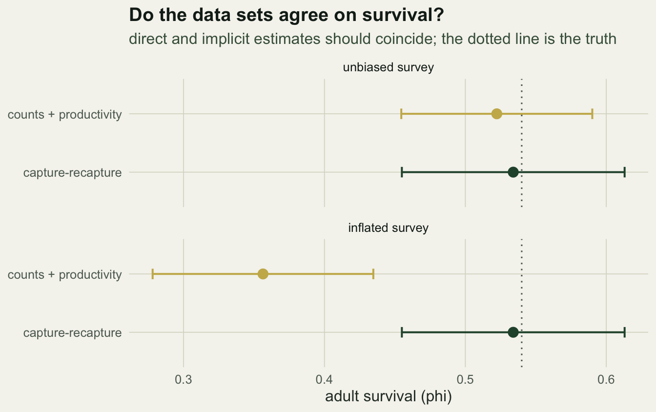
With the unbiased survey the two estimates sit on top of each other: capture-recapture gives survival 0.534 and the implicit route gives 0.522, a conflict score of 0.22, well within sampling noise. With the inflated survey the implicit survival collapses to 0.356, because the model must lower survival to reconcile the true count trajectory with an over-stated recruitment, while the capture-recapture estimate is untouched at 0.534. The conflict score is 3.13, far past the value that would prompt concern.

cf <- data.frame(
  survey = factor(rep(c("unbiased survey", "inflated survey"), each = 2),
                  levels = c("unbiased survey", "inflated survey")),
  source = rep(c("capture-recapture", "counts + productivity"), 2),
  est = c(phi_cr, im_ok["phi"], phi_cr, im_bi["phi"]),
  se  = c(se_cr, im_ok["se"], se_cr, im_bi["se"])
)
ggplot(cf, aes(est, source, colour = source)) +
  geom_vline(xintercept = phi_true, linetype = "dotted", colour = faint) +
  geom_errorbarh(aes(xmin = est - 1.96 * se, xmax = est + 1.96 * se),
                 height = 0.18, linewidth = 0.7) +
  geom_point(size = 3.2) +
  facet_wrap(~survey, ncol = 1) +
  scale_colour_manual(values = c("capture-recapture" = forest,
                                 "counts + productivity" = gold), guide = "none") +
  labs(x = "adult survival (phi)", y = NULL,
       title = "Do the data sets agree on survival?",
       subtitle = "direct and implicit estimates should coincide; the dotted line is the truth") +
  theme_te()

Warning: `geom_errorbarh()` was deprecated in ggplot2 4.0.0.
ℹ Please use the `orientation` argument of `geom_errorbar()` instead.

`height` was translated to `width`.

Figure 1: Adult survival estimated from capture-recapture (green) and implicitly from counts and productivity (gold), for an unbiased and an inflated productivity survey, with 95 per cent intervals. Under the unbiased survey the two agree. Under the inflated survey the implicit estimate drops well below the capture-recapture estimate: the data sets disagree, which is the signature of a violated assumption.

Why the count fit does not reveal it

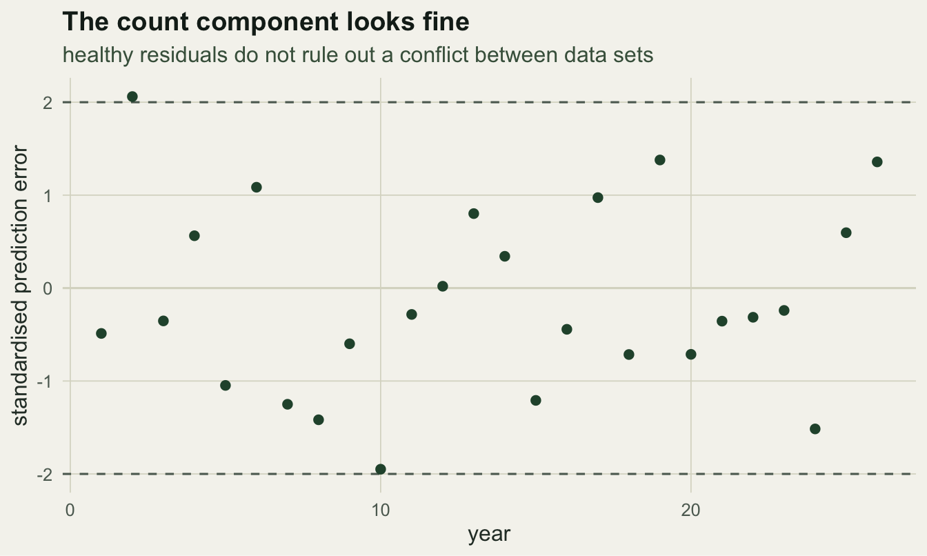
The natural worry is that this only shows up because we knew where to look. It does not show up, though, in the count component itself. Fit the full integrated model to the inflated data and inspect the standardised one-step prediction errors from the Kalman filter, the usual residual check for a state-space model.

of <- optim(c(qlogis(.5), log(.5), log(11), qlogis(.5), log(C[1])), function(pp)
  -(kf_ll(plogis(pp[1]), exp(pp[2]), exp(pp[3]), exp(pp[5])) +
    marray_ll(plogis(pp[1]), plogis(pp[4])) +
    sum(dpois(prodJ_bias, prodB * exp(pp[2]), log = TRUE))),
  method = "BFGS", control = list(reltol = 1e-11))
phi_f <- plogis(of$par[1]); f_f <- exp(of$par[2]); sy_f <- exp(of$par[3]); N1_f <- exp(of$par[5])
lam <- phi_f + f_f; dv <- phi_f * (1 - phi_f) + f_f; a <- N1_f; P <- (2 * sy_f)^2
innov <- numeric(Tyr)
for (t in 1:Tyr) {
  if (t > 1) { ap <- a; a <- lam * ap; P <- lam^2 * P + dv * max(ap, 1) }
  F <- P + sy_f^2; innov[t] <- (C[t] - a) / sqrt(F)
  K <- P / F; a <- a + K * (C[t] - a); P <- (1 - K) * P
}
rd <- data.frame(year = 1:Tyr, z = innov)
ggplot(rd, aes(year, z)) +
  geom_hline(yintercept = 0, colour = linec) +
  geom_hline(yintercept = c(-2, 2), linetype = "dashed", colour = faint) +
  geom_point(colour = forest, size = 2) +
  labs(x = "year", y = "standardised prediction error",
       title = "The count component looks fine",
       subtitle = "healthy residuals do not rule out a conflict between data sets") +
  theme_te()

Figure 2: Standardised one-step prediction errors from the full integrated model fitted to the inflated data, by year, with the plus or minus two band. They scatter around zero with roughly unit spread and no trend: the count component looks perfectly healthy. The mis-specification is invisible here and surfaces only in the cross-source comparison above.

The shared survival in that full fit comes out at 0.443, a compromise between the capture-recapture value and the depressed implicit value, and yet the residuals give no hint of trouble: 1 of 26 fall outside the two-sigma band, about what chance predicts. A model that fits its counts can still be built on data sets that contradict each other.

Takeaways

An integrated population model earns its precision by making data sets share parameters, and the same sharing lets a fault in one source travel into the estimates drawn from the others. Checking the model needs both halves: the component checks that any single-source analysis would use, and a cross-source test that the sources agree. Estimating a rate directly and implicitly and comparing them is a direct, cheap version of that test; a large gap points to a broken assumption, whether biased productivity, emigration mistaken for mortality, or an unmodelled trend. The count residuals here stayed clean while the two survival estimates were three standard errors apart, which is the lesson in one line: in a joint model, agreement between the data sets is a thing you must test for, not assume. That closes this series on integrated population models, from the first joint likelihood to the checks that keep it honest.

References

Besbeas, P. and Morgan, B. J. T. 2014. Goodness of fit of integrated population models using calibrated simulation. Methods in Ecology and Evolution 5(12):1373-1382 (10.1111/2041-210X.12279).

Abadi, F., Gimenez, O., Arlettaz, R. and Schaub, M. 2010. An assessment of integrated population models: bias, accuracy and violation of the assumption of independence. Ecology 91(1):7-14 (10.1890/08-2235.1).

Riecke, T. V., Williams, P. J., Behnke, T. L., Gibson, D., Leach, A. G., Sedinger, B. S., Street, P. A. and Sedinger, J. S. 2019. Integrated population models: model assumptions and inference. Methods in Ecology and Evolution 10(7):1072-1082 (10.1111/2041-210X.13195).

Conn, P. B., Johnson, D. S., Williams, P. J., Melin, S. R. and Hooten, M. B. 2018. A guide to Bayesian model checking for ecologists. Ecological Monographs 88(4):526-542 (10.1002/ecm.1314).

Schaub, M. and Abadi, F. 2011. Integrated population models: a novel analysis framework for deeper insights into population dynamics. Journal of Ornithology 152(S1):227-237 (10.1007/s10336-010-0632-7).

Kery, M. and Schaub, M. 2012. Bayesian Population Analysis using WinBUGS. Academic Press (ISBN 978-0-12-387020-9).

Related tutorials

• Integrated population models from scratch
• Implicit information in integrated models
• Demographic and environmental variance in an IPM
• Cormack-Jolly-Seber survival