---
title: "Implicit information in integrated models"
description: "How an integrated model estimates a demographic rate it has no direct data for, how much each data set contributes, and why implicit estimates lean on it."
date: "2026-05-21 10:00"
categories: [R, population dynamics, capture-recapture, demography, ecology tutorial]
image: thumbnail.png
image-alt: "A survival-recruitment likelihood plane with a diagonal ridge, and three coloured contours: capture-recapture alone and productivity alone each narrow the ridge to a long thin ellipse, and the two together to a shorter ellipse where those two overlap."
---
The previous post built an integrated population model (IPM) and showed that counts alone cannot separate adult survival from recruitment: the two lie anywhere along a ridge of constant growth rate. Adding capture-recapture and productivity data cut across that ridge and fixed both rates. This post looks at the mechanism more closely, and at a result that seems to give something for nothing: an IPM can estimate a rate for which it holds no direct data at all.
The reason is the shared trajectory. The counts fix the growth rate, which is survival plus recruitment. So if any one of the two rates is known, the other follows by subtraction. Capture-recapture data fix survival directly, and the counts then imply recruitment; a productivity survey fixes recruitment directly, and the counts then imply survival. This implicit information is real and useful, but it rests entirely on the demographic model being correct, and that is where the care comes in.
## Estimating a rate with no data for it
We simulate the same kind of population as before: annual counts, a capture-recapture study on adults, and a productivity survey. Then we fit the IPM four ways, dropping data sets to see what each one identifies.
```{r}
#| label: setup
#| code-fold: true
#| code-summary: "Setup: packages, colours and plot theme"
#| results: hide
#| message: false
#| warning: false
library(ggplot2)
paper <- "#f5f4ee"; ink <- "#16241d"; body <- "#2c3a31"; forest <- "#275139"
labelc <- "#46604a"; sage <- "#93a87f"; linec <- "#dad9ca"; faint <- "#5d6b61"
gold <- "#c9b458"; rust <- "#b5534e"
theme_te <- function(base_size = 12) {
  theme_minimal(base_size = base_size) +
    theme(
      plot.background  = element_rect(fill = paper, colour = NA),
      panel.background = element_rect(fill = paper, colour = NA),
      panel.grid.minor = element_blank(),
      panel.grid.major = element_line(colour = linec, linewidth = 0.3),
      axis.title = element_text(colour = body),
      axis.text  = element_text(colour = faint),
      plot.title = element_text(colour = ink, face = "bold"),
      plot.subtitle = element_text(colour = labelc),
      legend.title = element_text(colour = body),
      legend.text  = element_text(colour = body),
      strip.text   = element_text(colour = ink)
    )
}
```
```{r}
#| label: simulate
set.seed(132)
Tyr <- 25; phi_true <- 0.55; f_true <- 0.48; sy_true <- 11; N1_true <- 180
N <- numeric(Tyr); N[1] <- N1_true
for (t in 1:(Tyr - 1)) {
  N[t + 1] <- rbinom(1, N[t], phi_true) + rpois(1, f_true * N[t])
}
C <- round(rnorm(Tyr, N, sy_true))

p_true <- 0.5; Kcr <- 9; Rrel <- rep(30, Kcr - 1)
recaps <- vector("list", Kcr - 1); never <- integer(Kcr - 1)
for (i in 1:(Kcr - 1)) {
  alive <- rep(TRUE, Rrel[i]); fr <- integer(Rrel[i]); rc <- numeric(Kcr)
  for (t in (i + 1):Kcr) {
    alive <- alive & (runif(length(alive)) < phi_true)
    got   <- alive & (runif(length(alive)) < p_true) & (fr == 0); fr[got] <- t
  }
  for (t in (i + 1):Kcr) rc[t] <- sum(fr == t)
  recaps[[i]] <- rc; never[i] <- Rrel[i] - sum(fr > 0)
}
Jyr <- 10; prodB <- rep(40, Jyr); prodJ <- rpois(Jyr, prodB * f_true)

kf_ll <- function(phi, f, sy, N1, C) {
  lam <- phi + f; dv <- phi * (1 - phi) + f; a <- N1; P <- (2 * sy)^2; ll <- 0
  for (t in seq_along(C)) {
    if (t > 1) { ap <- a; a <- lam * ap; P <- lam^2 * P + dv * max(ap, 1) }
    Fv <- P + sy^2; ll <- ll + dnorm(C[t], a, sqrt(Fv), log = TRUE)
    K <- P / Fv; a <- a + K * (C[t] - a); P <- (1 - K) * P
  }
  ll
}
marray_ll <- function(phi, p) {
  ll <- 0
  for (i in 1:(Kcr - 1)) {
    ts <- (i + 1):Kcr; q <- phi^(ts - i) * (1 - p)^(ts - i - 1) * p
    ll <- ll + sum(recaps[[i]][ts] * log(q)) + never[i] * log(1 - sum(q))
  }
  ll
}
```
```{r}
#| label: fits
fitv <- function(use) {
  has_p <- "cr" %in% use
  init <- if (has_p) c(qlogis(.5), log(.5), log(12), qlogis(.5), log(C[1]))
          else       c(qlogis(.5), log(.5), log(12), log(C[1]))
  fn <- function(par) {
    phi <- plogis(par[1]); ff <- exp(par[2]); sy <- exp(par[3])
    if (has_p) { p <- plogis(par[4]); N1 <- exp(par[5]) } else { N1 <- exp(par[4]) }
    ll <- 0
    if ("count" %in% use) ll <- ll + kf_ll(phi, ff, sy, N1, C)
    if ("cr"    %in% use) ll <- ll + marray_ll(phi, p)
    if ("prod"  %in% use) ll <- ll + sum(dpois(prodJ, prodB * ff, log = TRUE))
    -ll
  }
  o <- optim(init, fn, method = "BFGS", hessian = TRUE,
             control = list(maxit = 1500, reltol = 1e-11))
  V <- solve(o$hessian); phi <- plogis(o$par[1]); ff <- exp(o$par[2])
  c(phi = phi, f = ff, se_phi = sqrt(V[1, 1]) * phi * (1 - phi), se_f = sqrt(V[2, 2]) * ff)
}
cr   <- fitv(c("count", "cr"))       # counts + capture-recapture (no productivity)
prod <- fitv(c("count", "prod"))     # counts + productivity (no capture-recapture)
full <- fitv(c("count", "cr", "prod"))
```
Fit the counts together with the capture-recapture data but no productivity survey. Recruitment `f` is estimated at `r round(cr["f"], 3)` (SE `r round(cr["se_f"], 3)`, true `r f_true`), even though not one recruit was counted: the capture-recapture data give survival, the counts give the growth rate, and recruitment falls out as the difference. The mirror image holds when we fit the counts with the productivity survey but no capture-recapture data: adult survival comes out at `r round(prod["phi"], 3)` (SE `r round(prod["se_phi"], 3)`, true `r phi_true`), with no marked animal ever re-encountered.
## How much each data set contributes
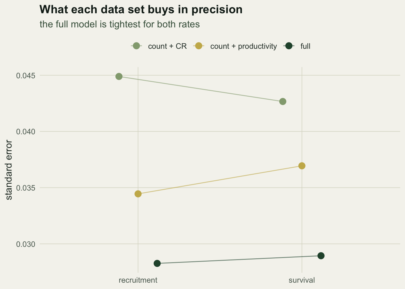
The implicit estimates are not free of cost. Within any one fit, the rate that has no data of its own comes out slightly less precise than the rate that does, and the full model, using every source, is the most precise of all.
```{r}
#| label: fig-precision
#| fig-cap: "Standard errors for adult survival and recruitment under three model fits. Each single-auxiliary fit identifies both rates (one directly, one implicitly through the shared trajectory), but the full model, drawing on counts, capture-recapture and productivity together, gives the tightest estimate of each."
#| fig-alt: "A grouped point-and-line chart with survival and recruitment on the x-axis and standard error on the y-axis; three coloured series for count-plus-CR, count-plus-productivity and full, with the full series lowest for both rates."
#| fig-width: 7
#| fig-height: 5
sedf <- data.frame(
  model = rep(c("count + CR", "count + productivity", "full"), each = 2),
  rate  = rep(c("survival", "recruitment"), 3),
  se    = c(cr["se_phi"], cr["se_f"], prod["se_phi"], prod["se_f"], full["se_phi"], full["se_f"])
)
sedf$model <- factor(sedf$model, levels = c("count + CR", "count + productivity", "full"))
ggplot(sedf, aes(rate, se, colour = model, group = model)) +
  geom_line(position = position_dodge(0.35), linewidth = 0.5, alpha = 0.6) +
  geom_point(position = position_dodge(0.35), size = 3.4) +
  scale_colour_manual(values = c("count + CR" = sage,
                                 "count + productivity" = gold, "full" = forest)) +
  labs(x = NULL, y = "standard error", colour = NULL,
       title = "What each data set buys in precision",
       subtitle = "the full model is tightest for both rates") +
  theme_te() + theme(legend.position = "top")
```
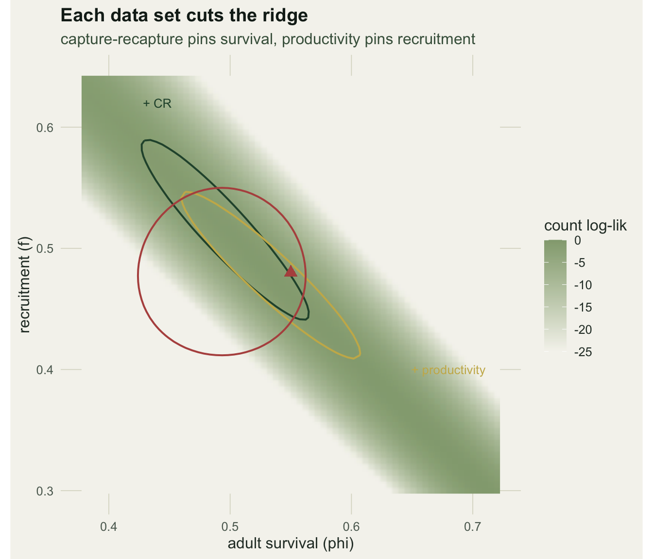
That comparison has to be made inside a fit, not across fits. In the count-plus-capture-recapture fit, survival has its own data and comes out at SE `r round(cr["se_phi"], 3)` while implicit recruitment costs `r round(cr["se_f"], 3)`; in the count-plus-productivity fit, recruitment is direct at `r round(prod["se_f"], 3)` and implicit survival costs `r round(prod["se_phi"], 3)`. Compare across fits and the ordering flips: implicit survival at `r round(prod["se_phi"], 3)` beats the `r round(cr["se_phi"], 3)` the capture-recapture data deliver directly, because the productivity survey is simply the stronger auxiliary data set here and its precision reaches survival through the growth-rate constraint. The full model tightens survival to `r round(full["se_phi"], 3)`. The geometry behind this is the ridge from the previous post. Each data set adds a constraint that cuts across it, and where the constraints meet is where the rates are pinned.
```{r}
#| label: fig-regions
#| fig-cap: "Likelihood over the survival-recruitment plane. The pale-to-dark shading is the count-only likelihood, a diagonal ridge of constant growth rate. Coloured contours mark where adding capture-recapture (which constrains survival) or productivity (which constrains recruitment) confines the fit; the two together (full) pin a small patch at the truth (rust)."
#| fig-alt: "A shaded square over survival and recruitment with a dark diagonal ridge running from the top left to the bottom right; two long narrow contours, one from capture-recapture and one from productivity, lie along the ridge and cut it short, and a smaller closed contour for the two together sits where they overlap near a rust triangle marking the truth."
#| fig-width: 7
#| fig-height: 6
# refit full with a fixed-p variant to get the nuisances and p for the surfaces
oful <- optim(c(qlogis(.5), log(.5), log(12), qlogis(.5), log(C[1])), function(par) {
  -(kf_ll(plogis(par[1]), exp(par[2]), exp(par[3]), exp(par[5]), C) +
    marray_ll(plogis(par[1]), plogis(par[4])) +
    sum(dpois(prodJ, prodB * exp(par[2]), log = TRUE)))
}, method = "BFGS", control = list(maxit = 1500, reltol = 1e-11))
syf <- exp(oful$par[3]); N1f <- exp(oful$par[5]); pf <- plogis(oful$par[4])
pg <- seq(0.38, 0.72, length.out = 70); fg <- seq(0.30, 0.64, length.out = 70)
gr <- expand.grid(phi = pg, f = fg)
gr$count <- mapply(function(a, b) kf_ll(a, b, syf, N1f, C), gr$phi, gr$f)
gr$cr    <- gr$count + sapply(gr$phi, function(a) marray_ll(a, pf))
gr$prod  <- gr$count + sapply(gr$f, function(b) sum(dpois(prodJ, prodB * b, log = TRUE)))
gr$fulls <- gr$cr + gr$prod - gr$count       # counts once, plus both auxiliary terms
gr$rz <- gr$count - max(gr$count); gr$rz[gr$rz < -25] <- -25
lev <- function(z) max(z) - 2
ggplot(gr, aes(phi, f)) +
  geom_raster(aes(fill = rz), interpolate = TRUE) +
  scale_fill_gradient(low = paper, high = sage, name = "count log-lik") +
  geom_contour(aes(z = cr),    breaks = lev(gr$cr),    colour = forest, linewidth = 0.7) +
  geom_contour(aes(z = prod),  breaks = lev(gr$prod),  colour = gold,   linewidth = 0.7) +
  geom_contour(aes(z = fulls), breaks = lev(gr$fulls), colour = rust,   linewidth = 0.7) +
  annotate("point", x = phi_true, y = f_true, colour = rust, size = 3, shape = 17) +
  annotate("text", x = 0.44, y = 0.62, label = "+ CR", colour = forest, size = 3.4) +
  annotate("text", x = 0.68, y = 0.40, label = "+ productivity", colour = gold, size = 3.4) +
  coord_equal() +
  labs(x = "adult survival (phi)", y = "recruitment (f)",
       title = "Each data set cuts the ridge",
       subtitle = "capture-recapture pins survival, productivity pins recruitment") +
  theme_te()
```
## The catch: implicit means model-dependent
Implicit information comes from forcing the counts and the auxiliary data to agree through the demographic model. If that model is wrong, the implicit estimate absorbs the error. Suppose the productivity survey is biased high, as happens when the monitored nests are easier to find and more successful than average. Fit counts and the inflated productivity together, with no capture-recapture data to anchor survival.
```{r}
#| label: bias
prodJ_bias <- rpois(Jyr, prodB * f_true * 1.3)          # productivity over-recorded by 30%
ob <- optim(c(qlogis(.5), log(.5), log(12), log(C[1])), function(par) {
  -(kf_ll(plogis(par[1]), exp(par[2]), exp(par[3]), exp(par[4]), C) +
    sum(dpois(prodJ_bias, prodB * exp(par[2]), log = TRUE)))
}, method = "BFGS", control = list(maxit = 1500, reltol = 1e-11))
phi_bias <- plogis(ob$par[1]); f_bias <- exp(ob$par[2])
```
The inflated productivity pushes recruitment up to `r round(f_bias, 3)`, and because the counts fix the growth rate, the implicit survival is dragged down to `r round(phi_bias, 3)`, well below the true `r phi_true`. Nothing in this fit looks wrong: the counts are matched and recruitment agrees with its (biased) survey. The error only shows if a second source disagrees. Here the capture-recapture data would put survival near `r round(full["phi"], 3)`, so the implicit and the direct survival estimates conflict, and that conflict is the signal that a demographic assumption has failed. Diagnosing this kind of hidden disagreement between data sets is the subject of the checking post later in this series.
## Takeaways
An integrated population model shares the growth rate across its data sets, so knowing one vital rate implies the other. That is why the model can report a survival probability with no marked animals and a recruitment rate with no offspring counts: the missing rate is recovered implicitly from the trajectory. The implicit estimate is genuine, and its precision can rival a direct estimate from a modest auxiliary survey, but it is only as trustworthy as the process model it leans on. A biased productivity survey quietly biases the implicit survival, and the giveaway is a clash with a second, direct estimate. The next post turns to a different question the IPM answers well: separating the year-to-year variability in the rates from the demographic noise of a finite population.
```{r}
#| label: thumb
#| include: false
th <- ggplot(gr, aes(phi, f)) +
geom_raster(aes(fill = rz), interpolate = TRUE) +
scale_fill_gradient(low = paper, high = sage, guide = "none") +
geom_contour(aes(z = cr), breaks = lev(gr$cr), colour = forest, linewidth = 0.8) +
geom_contour(aes(z = prod), breaks = lev(gr$prod), colour = gold, linewidth = 0.8) +
geom_contour(aes(z = fulls), breaks = lev(gr$fulls), colour = rust, linewidth = 0.8) +
coord_equal() + labs(x = NULL, y = NULL) + theme_te()
ggsave("thumbnail.png", th, width = 7.5, height = 5.4, dpi = 100, bg = paper)
```
## References
Besbeas P, Freeman SN, Morgan BJT, Catchpole EA 2002 Biometrics 58(3):540-547 (10.1111/j.0006-341X.2002.00540.x)
Schaub M, Abadi F 2011 Journal of Ornithology 152(S1):227-237 (10.1007/s10336-010-0632-7)
Abadi F, Gimenez O, Arlettaz R, Schaub M 2010 Ecology 91(1):7-14 (10.1890/08-2235.1)
Riecke TV, Williams PJ, Behnke TL, Gibson D, Leach AG, Sedinger BS, Street PA, Sedinger JS 2019 Methods in Ecology and Evolution 10(7):1072-1082 (10.1111/2041-210X.13195)
Zipkin EF, Saunders SP 2018 Biological Conservation 217:240-250 (10.1016/j.biocon.2017.10.017)
Kery M, Schaub M 2012 Bayesian Population Analysis using WinBUGS. Academic Press (ISBN 978-0-12-387020-9)
## Related tutorials
- [Integrated population models from scratch](../integrated-population-model-basics/)
- [Cormack-Jolly-Seber survival](../cormack-jolly-seber-survival/)
- [Nest survival and logistic exposure](../nest-survival-logistic-exposure/)
- [Estimating population trend](../population-trend-estimation/)