---
title: "Integrated population models from scratch"
description: "Integrated population models in base R: joining counts, capture-recapture and productivity, and why counts alone cannot split survival from recruitment."
date: "2026-05-21 09:00"
categories: [R, population dynamics, capture-recapture, demography, ecology tutorial]
image: thumbnail.png
image-alt: "A declining count time series shown as dark points, with a reconstructed abundance trajectory drawn as a line inside a shaded uncertainty band. The line falls from about 190 at the first of twenty five time points to a low near the tenth, rebounds to a smaller peak around the sixteenth, then drops to about 80 at the end."
---
A monitoring programme rarely gives you one clean picture of a population. Annual counts show that numbers are falling, but not why: is adult survival low, or is recruitment failing? A capture-recapture study on marked adults estimates survival, but says nothing about how many animals there are. A productivity survey counts offspring per adult, but leaves both abundance and survival open. Each data set answers part of the question and leaves the rest unidentifiable.
An integrated population model (IPM) fits all of these at once. It writes a single likelihood that is the sum of the pieces from each data set, tied together by shared demographic parameters and a projection that steps abundance forward. The counts constrain the trajectory, the capture-recapture data pin survival, the productivity survey pins recruitment, and because they share the same rates, each source sharpens the others. This post builds a maximum-likelihood IPM from scratch in base R, following the Kalman-filter formulation of Besbeas et al. (2002), and shows the central payoff: what the counts cannot do alone.
## Three data sets, one population
Consider a population censused once a year before breeding, with `N_t` adult females. Two rates drive it. Adults survive to the next year with probability `phi`, and each adult contributes on average `f` recruits that enter the population as new adults the following year (a lumped fecundity times first-year survival). The expected next-year size is `(phi + f)` times the current size, so the growth rate is `phi + f`. A declining population has `phi + f` below one, but that single number does not tell you whether the shortfall is in survival or in recruitment.
The process carries demographic stochasticity. Survivors are a binomial draw and recruits a Poisson draw, so the next state has mean `(phi + f) N_t` and a variance that grows with `N_t`: `N_t` times `phi(1 - phi) + f`. We observe the state with error through the annual counts, and we bring in two auxiliary data sets: a capture-recapture study that marks and re-encounters adults, and a productivity survey that counts recruits produced by a sample of adults.
```{r}
#| label: setup
#| code-fold: true
#| code-summary: "Setup: packages, colours and plot theme"
#| results: hide
#| message: false
#| warning: false
library(ggplot2)
paper <- "#f5f4ee"; ink <- "#16241d"; body <- "#2c3a31"; forest <- "#275139"
labelc <- "#46604a"; sage <- "#93a87f"; linec <- "#dad9ca"; faint <- "#5d6b61"
gold <- "#c9b458"; rust <- "#b5534e"
theme_te <- function(base_size = 12) {
  theme_minimal(base_size = base_size) +
    theme(
      plot.background  = element_rect(fill = paper, colour = NA),
      panel.background = element_rect(fill = paper, colour = NA),
      panel.grid.minor = element_blank(),
      panel.grid.major = element_line(colour = linec, linewidth = 0.3),
      axis.title = element_text(colour = body),
      axis.text  = element_text(colour = faint),
      plot.title = element_text(colour = ink, face = "bold"),
      plot.subtitle = element_text(colour = labelc),
      legend.title = element_text(colour = body),
      legend.text  = element_text(colour = body),
      strip.text   = element_text(colour = ink)
    )
}
```
```{r}
#| label: simulate
set.seed(131)
Tyr <- 25; phi_true <- 0.52; f_true <- 0.45; sy_true <- 12; N1_true <- 200

# true demographic process: survivors Binomial, recruits Poisson
N <- numeric(Tyr); N[1] <- N1_true
for (t in 1:(Tyr - 1)) {
  S <- rbinom(1, N[t], phi_true)
  R <- rpois(1, f_true * N[t])
  N[t + 1] <- S + R
}
C <- round(rnorm(Tyr, N, sy_true))                 # annual counts (with error)

# capture-recapture: individual CJS histories collapsed to an m-array
p_true <- 0.5; Kcr <- 9; Rrel <- rep(30, Kcr - 1)
recaps <- vector("list", Kcr - 1); never <- integer(Kcr - 1)
for (i in 1:(Kcr - 1)) {
  alive <- rep(TRUE, Rrel[i]); fr <- integer(Rrel[i]); rc <- numeric(Kcr)
  for (t in (i + 1):Kcr) {
    alive <- alive & (runif(length(alive)) < phi_true)
    got   <- alive & (runif(length(alive)) < p_true) & (fr == 0)
    fr[got] <- t
  }
  for (t in (i + 1):Kcr) rc[t] <- sum(fr == t)
  recaps[[i]] <- rc; never[i] <- Rrel[i] - sum(fr > 0)
}

# productivity survey: recruits from a sample of adults, J years
Jyr <- 10; prodB <- rep(40, Jyr); prodJ <- rpois(Jyr, prodB * f_true)
```
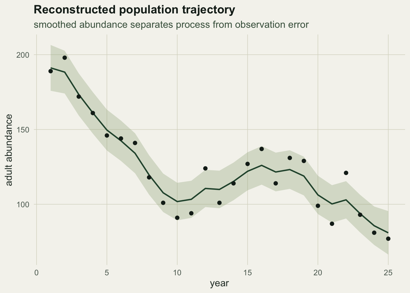
The counts fall from `r C[1]` to `r C[Tyr]` over `r Tyr` years, a decline of roughly `r round(100 * (1 - (C[Tyr] / C[1])^(1 / (Tyr - 1))), 1)` per cent a year. On their own they cannot say where the loss sits.
## One likelihood from three pieces
Each data set contributes a log-likelihood, and the IPM adds them. For the counts we use the Kalman filter: the demographic mean and its state-dependent variance define a linear Gaussian state-space, so the count log-likelihood is the sum of the one-step prediction densities (Besbeas et al. 2002). For the capture-recapture data we use the standard m-array multinomial: an animal released at occasion `i` and first seen again at `t` contributes `phi^(t-i) (1-p)^(t-i-1) p`, and the never-seen cell closes each row. For productivity we use a Poisson likelihood for recruits given the number of adults surveyed. Survival `phi` is shared between the counts and the capture-recapture data; recruitment `f` is shared between the counts and the productivity survey.
```{r}
#| label: likelihood
# count component: Kalman filter with a state-dependent process variance
kf_ll <- function(phi, f, sy, N1, C) {
  lam <- phi + f; dv <- phi * (1 - phi) + f
  a <- N1; P <- (2 * sy)^2; ll <- 0
  for (t in seq_along(C)) {
    if (t > 1) { ap <- a; a <- lam * ap; P <- lam^2 * P + dv * max(ap, 1) }
    Fv <- P + sy^2
    ll <- ll + dnorm(C[t], a, sqrt(Fv), log = TRUE)
    K <- P / Fv; a <- a + K * (C[t] - a); P <- (1 - K) * P
  }
  ll
}
# capture-recapture component: m-array multinomial
marray_ll <- function(phi, p) {
  ll <- 0
  for (i in 1:(Kcr - 1)) {
    ts <- (i + 1):Kcr
    q  <- phi^(ts - i) * (1 - p)^(ts - i - 1) * p
    ll <- ll + sum(recaps[[i]][ts] * log(q)) + never[i] * log(1 - sum(q))
  }
  ll
}
# joint negative log-likelihood (drop components via `use` to see their effect)
nll <- function(par, use = c("count", "cr", "prod")) {
  phi <- plogis(par[1]); f <- exp(par[2]); sy <- exp(par[3])
  p   <- plogis(par[4]); N1 <- exp(par[5]); ll <- 0
  if ("count" %in% use) ll <- ll + kf_ll(phi, f, sy, N1, C)
  if ("cr"    %in% use) ll <- ll + marray_ll(phi, p)
  if ("prod"  %in% use) ll <- ll + sum(dpois(prodJ, prodB * f, log = TRUE))
  -ll
}

st  <- c(qlogis(0.5), log(0.5), log(15), qlogis(0.5), log(C[1]))
fit <- optim(st, nll, use = c("count", "cr", "prod"),
             method = "BFGS", hessian = TRUE,
             control = list(maxit = 1000, reltol = 1e-11))
stopifnot(fit$convergence == 0)   # check before inverting the Hessian
V     <- solve(fit$hessian); pr <- fit$par
phi_h <- plogis(pr[1]); f_h <- exp(pr[2]); sy_h <- exp(pr[3])
p_h   <- plogis(pr[4]); N1_h <- exp(pr[5])
se_phi <- sqrt(V[1, 1]) * phi_h * (1 - phi_h)
se_f   <- sqrt(V[2, 2]) * f_h
```
The joint fit recovers both rates: survival `phi` is `r round(phi_h, 3)` (SE `r round(se_phi, 3)`, true `r phi_true`) and recruitment `f` is `r round(f_h, 3)` (SE `r round(se_f, 3)`, true `r f_true`). The implied growth rate is `r round(phi_h + f_h, 3)`, and the observation standard deviation comes out at `r round(sy_h, 1)`. Each rate has a tight standard error, because the capture-recapture data speak directly to `phi` and the productivity survey directly to `f`, while the counts tie both to the abundance trajectory.
## Why the counts alone cannot split the rates
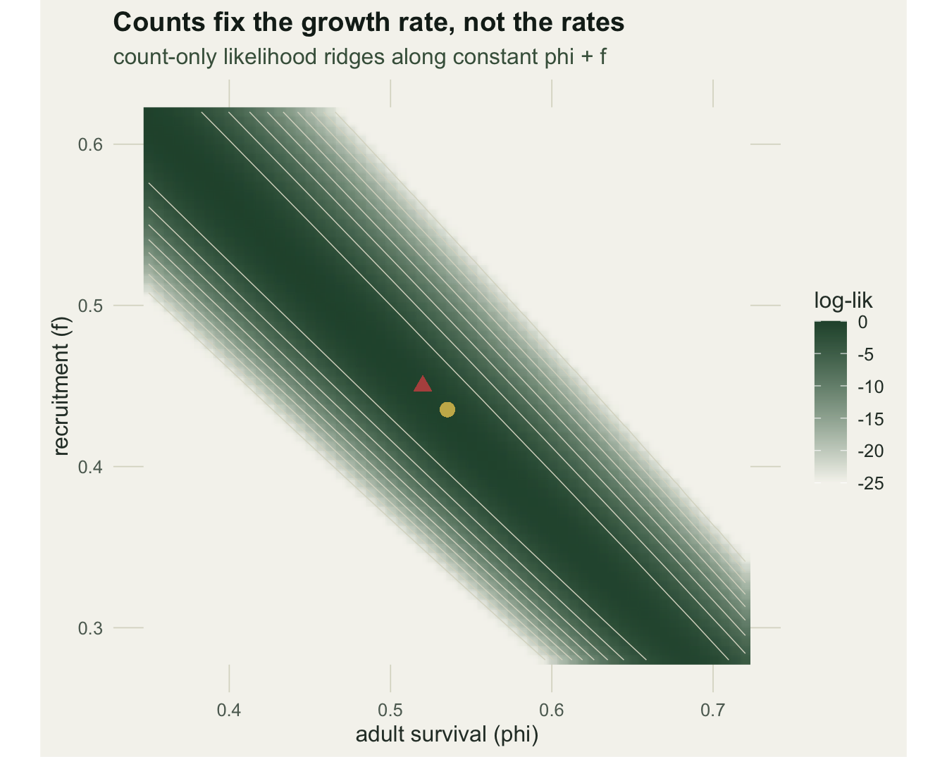
Drop the capture-recapture and productivity pieces and fit the counts on their own. The count likelihood depends on survival and recruitment almost entirely through their sum, the growth rate, so it can estimate `phi + f` but not the two rates separately. Profiling the count-only likelihood over `phi` (re-optimising the other parameters at each value) traces a nearly flat ridge; the joint likelihood, with the two auxiliary data sets attached, peaks sharply.
```{r}
#| label: ridge-profile
phi_grid <- seq(0.32, 0.74, by = 0.015)
prof <- function(phi_fix, use) {
  o <- optim(c(log(0.5), log(15), qlogis(0.5), log(C[1])), function(pp) {
    f <- exp(pp[1]); sy <- exp(pp[2]); p <- plogis(pp[3]); N1 <- exp(pp[4]); ll <- 0
    if ("count" %in% use) ll <- ll + kf_ll(phi_fix, f, sy, N1, C)
    if ("cr"    %in% use) ll <- ll + marray_ll(phi_fix, p)
    if ("prod"  %in% use) ll <- ll + sum(dpois(prodJ, prodB * f, log = TRUE))
    -ll
  }, method = "Nelder-Mead", control = list(maxit = 2000))
  -o$value
}
ll_count <- sapply(phi_grid, prof, use = "count")
ll_joint <- sapply(phi_grid, prof, use = c("count", "cr", "prod"))
w_count <- range(phi_grid[ll_count >= max(ll_count) - 2])
w_joint <- range(phi_grid[ll_joint >= max(ll_joint) - 2])
```
Within two log-likelihood units of its maximum, the count-only profile admits survival anywhere from `r round(w_count[1], 2)` to `r round(w_count[2], 2)`, the full width of the plausible range: the data cannot choose. The joint profile narrows that to [`r round(w_joint[1], 2)`, `r round(w_joint[2], 2)`]. The ridge is clearest as a surface. Fixing the observation error and starting abundance at their fitted values, the count-only log-likelihood over the survival-recruitment plane runs along the anti-diagonal where `phi + f` is constant.
```{r}
#| label: fig-ridge
#| fig-cap: "Count-only log-likelihood over the survival and recruitment plane (pale to dark), with observation error and initial abundance fixed at their fitted values. The likelihood forms a diagonal ridge of constant growth rate: the counts fix the sum but not the split. The joint estimate (gold) and the truth (rust) sit where the auxiliary data pin a single point."
#| fig-alt: "A shaded square panel over survival on the x-axis and recruitment on the y-axis, with a dark diagonal band running from upper-left to lower-right marking equal growth rate; a gold point and a rust point sit close together on the band."
#| fig-width: 7
#| fig-height: 5.6
pg <- seq(0.35, 0.72, length.out = 60)
fg <- seq(0.28, 0.62, length.out = 60)
gr <- expand.grid(phi = pg, f = fg)
gr$ll <- mapply(function(ph, ff) kf_ll(ph, ff, sy_h, N1_h, C), gr$phi, gr$f)
gr$ll <- gr$ll - max(gr$ll)
gr$ll[gr$ll < -25] <- -25
ggplot(gr, aes(phi, f)) +
  geom_raster(aes(fill = ll), interpolate = TRUE) +
  geom_contour(aes(z = ll), colour = linec, linewidth = 0.25, bins = 10) +
  annotate("point", x = phi_h, y = f_h, colour = gold, size = 3) +
  annotate("point", x = phi_true, y = f_true, colour = rust, size = 3, shape = 17) +
  scale_fill_gradient(low = paper, high = forest, name = "log-lik") +
  coord_equal() +
  labs(x = "adult survival (phi)", y = "recruitment (f)",
       title = "Counts fix the growth rate, not the rates",
       subtitle = "count-only likelihood ridges along constant phi + f") +
  theme_te()
```
The joint model lands on a single point because the capture-recapture data cut across the ridge (they constrain `phi` regardless of `f`) and the productivity survey constrains `f`. With survival and recruitment identified, the Kalman smoother reconstructs the abundance trajectory that generated the counts.
```{r}
#| label: fig-trajectory
#| fig-cap: "Annual counts (points) and the Kalman-smoothed abundance reconstructed by the fitted IPM (line and shaded 95 per cent band). The smoother separates observation error from the demographic process, so the trajectory is steadier than the raw counts while still tracking the decline the vital rates imply."
#| fig-alt: "A time series over 25 years: scattered dark points for the annual counts fall from about 190 to 80, with a smooth green line and a pale ribbon threading through them, declining overall with a rebound near year sixteen."
#| fig-width: 7
#| fig-height: 5
lam <- phi_h + f_h; dv <- phi_h * (1 - phi_h) + f_h
ap <- Pp <- af <- Pf <- numeric(Tyr)
a <- N1_h; P <- (2 * sy_h)^2
for (t in 1:Tyr) {
  if (t > 1) { a <- lam * af[t - 1]; P <- lam^2 * Pf[t - 1] + dv * max(af[t - 1], 1) }
  ap[t] <- a; Pp[t] <- P
  Fk <- P + sy_h^2; K <- P / Fk
  af[t] <- a + K * (C[t] - a); Pf[t] <- (1 - K) * P
}
as_ <- af; Ps <- Pf                                   # RTS smoother (backward)
for (t in (Tyr - 1):1) {
  J <- Pf[t] * lam / Pp[t + 1]
  as_[t] <- af[t] + J * (as_[t + 1] - ap[t + 1])
  Ps[t]  <- Pf[t] + J^2 * (Ps[t + 1] - Pp[t + 1])
}
td <- data.frame(year = 1:Tyr, count = C, Nsm = as_,
                 lo = as_ - 1.96 * sqrt(Ps), hi = as_ + 1.96 * sqrt(Ps))
ggplot(td, aes(year)) +
  geom_ribbon(aes(ymin = lo, ymax = hi), fill = sage, alpha = 0.3) +
  geom_line(aes(y = Nsm), colour = forest, linewidth = 0.8) +
  geom_point(aes(y = count), colour = ink, size = 1.8) +
  labs(x = "year", y = "adult abundance",
       title = "Reconstructed population trajectory",
       subtitle = "smoothed abundance separates process from observation error") +
  theme_te()
```
## Takeaways
An integrated population model is less an algorithm than an accounting rule: write the likelihood each data set would contribute on its own, make them share the demographic parameters, and add them up. Here three pieces, a Kalman filter for the counts, an m-array multinomial for the capture-recapture data, and a Poisson term for productivity, combine into one `optim` call with no specialised software. The gain is identifiability. Counts alone estimate the growth rate but leave survival and recruitment lying anywhere along a ridge; the auxiliary data cut across it and fix both, and the smoother then reconstructs abundance with observation error stripped out. The next post looks more closely at what each data set contributes, including the surprising fact that an IPM can estimate a rate for which it holds no direct data at all.
```{r}
#| label: thumb
#| include: false
th <- ggplot(td, aes(year)) +
geom_ribbon(aes(ymin = lo, ymax = hi), fill = sage, alpha = 0.3) +
geom_line(aes(y = Nsm), colour = forest, linewidth = 0.9) +
geom_point(aes(y = count), colour = ink, size = 1.6) +
labs(x = NULL, y = NULL) + theme_te() +
theme(legend.position = "none")
ggsave("thumbnail.png", th, width = 7.5, height = 5.4, dpi = 100, bg = paper)
```
## References
Besbeas P, Freeman SN, Morgan BJT, Catchpole EA 2002 Biometrics 58(3):540-547 (10.1111/j.0006-341X.2002.00540.x)
Brooks SP, King R, Morgan BJT 2004 Animal Biodiversity and Conservation 27(1):515-529 (10.32800/abc.2004.27.0515)
Schaub M, Abadi F 2011 Journal of Ornithology 152(S1):227-237 (10.1007/s10336-010-0632-7)
Abadi F, Gimenez O, Arlettaz R, Schaub M 2010 Ecology 91(1):7-14 (10.1890/08-2235.1)
Zipkin EF, Saunders SP 2018 Biological Conservation 217:240-250 (10.1016/j.biocon.2017.10.017)
Kery M, Schaub M 2012 Bayesian Population Analysis using WinBUGS. Academic Press. ISBN 978-0-12-387020-9
## Related tutorials
- [Cormack-Jolly-Seber survival](../cormack-jolly-seber-survival/)
- [The Gompertz state-space model](../gompertz-state-space-model/)
- [Estimating population trend](../population-trend-estimation/)
- [Leslie matrix population models](../leslie-matrix-population-models/)