---
title: "Gompertz state-space model in R"
description: "Separating process noise from observation error in a population time series with a Gompertz state-space model in R, fitted by a hand-coded Kalman filter."
date: "2026-05-15 09:00"
categories: [R, population dynamics, time series, state-space models, density dependence, ecology tutorial]
image: thumbnail.png
image-alt: "A hidden log-abundance trajectory, noisy observed counts around it, and a state-space estimate that tracks the hidden state."
---
The [test for density dependence](../detecting-density-dependence/) works on true abundances, but real counts carry sampling error. That error is not harmless. When the counts feeding a Gompertz regression are noisy, the density-dependence slope is pulled downwards, so a population is made to look more tightly regulated than it is. The Gompertz state-space model fixes the diagnosis by treating the true abundance as a hidden state and the counts as noisy observations of it, then estimating the process noise and the observation error separately. This post fits that model in base R with a Kalman filter written by hand, shows how much bias it removes, and shows why the split between the two error sources is hard to pin down.
## Two sources of variation
The model has two layers. A hidden process describes the real log abundance, and an observation layer describes what gets counted:
$$X_{t+1} = a + b\,X_t + \varepsilon_t, \quad \varepsilon_t \sim \mathrm{Normal}(0, \sigma_p^2),$$
$$Y_t = X_t + \eta_t, \quad \eta_t \sim \mathrm{Normal}(0, \sigma_o^2).$$
Here $X_t$ is the true log abundance, hidden from view, and $Y_t$ is the observed log count. The process variance $\sigma_p^2$ is genuine population fluctuation; the observation variance $\sigma_o^2$ is counting error. The slope $b$ still measures density dependence exactly as before, with $b < 1$ meaning regulation. The problem with the naive regression from the previous post is that it treats $Y_t$ as if it were $X_t$, so the noise in the predictor drags the estimated slope towards zero.
```{r}
#| label: setup
#| code-fold: true
#| code-summary: "Setup: packages, colours and plot theme"
#| results: hide
#| message: false
#| warning: false
suppressPackageStartupMessages({library(ggplot2); library(dplyr); library(tidyr)})
ink<-"#16241d"; body<-"#2c3a31"; forest<-"#275139"; gold<-"#c9b458"
paper<-"#f5f4ee"; line<-"#dad9ca"; faint<-"#5d6b61"; aban<-"#b5534e"; mown<-"#2f8f63"
theme_te <- function(){
  theme_minimal(base_size=12)+
  theme(plot.background=element_rect(fill=paper,colour=NA),
        panel.background=element_rect(fill=paper,colour=NA),
        panel.grid.minor=element_blank(),
        panel.grid.major=element_line(colour=line,linewidth=.3),
        axis.title=element_text(colour=ink), axis.text=element_text(colour=faint),
        plot.title=element_text(colour=ink,size=12,face="bold"),
        strip.text=element_text(colour=ink,face="bold"),
        legend.position="bottom", legend.title=element_text(colour=ink),
        legend.text=element_text(colour=body))
}
```
## The Kalman filter likelihood
A linear Gaussian state-space model has a likelihood that the Kalman filter computes exactly. The filter sweeps through the years, and at each step it holds a prediction of the hidden state and its variance. It compares that prediction with the new observation, and the mismatch, weighted by how much to trust the observation, both updates the state estimate and contributes to the log-likelihood. The recursion is short enough to write out in full.
```{r}
#| label: helpers
kf_nll <- function(par, y, fixed_so2=NA){
  a<-par[1]; b<-tanh(par[2]); sp2<-exp(par[3])
  so2 <- if(is.na(fixed_so2)) exp(par[4]) else fixed_so2
  n_t<-length(y); xp<-a/(1-b); Pp<-sp2/(1-b^2); ll<-0
  for(t in 1:n_t){
    v<-y[t]-xp; S<-Pp+so2; K<-Pp/S      # innovation, its variance, Kalman gain
    xf<-xp+K*v; Pf<-(1-K)*Pp            # filtered state and variance
    ll<-ll-0.5*(log(2*pi*S)+v*v/S)      # log-likelihood contribution
    xp<-a+b*xf; Pp<-b^2*Pf+sp2          # predict the next state
  }
  -ll
}
fit_gss <- function(y){
  n<-length(y); x0<-y[-n]; x1<-y[-1]; b0<-cov(x0,x1)/var(x0); a0<-mean(x1)-b0*mean(x0)
  vr<-var(x1-(a0+b0*x0)); b0<-min(max(b0,-0.9),0.9)
  st<-c(a0, atanh(b0), log(0.5*vr), log(0.5*vr))
  op<-optim(st, kf_nll, y=y, method="BFGS", hessian=TRUE, control=list(maxit=1000))
  b<-tanh(op$par[2]); V<-tryCatch(solve(op$hessian), error=function(e) matrix(NA,4,4))
  se_tb<-sqrt(V[2,2])
  list(a=op$par[1], b=b, sp=sqrt(exp(op$par[3])), so=sqrt(exp(op$par[4])),
       theta_b=op$par[2], se_tb=se_tb, se_b=(1-b^2)*se_tb, conv=op$convergence, ll=-op$value)
}
naive_b <- function(y){ n<-length(y); cov(y[-n],y[-1])/var(y[-n]) }
kf_smooth <- function(y,a,b,sp2,so2){ n_t<-length(y)
  xp<-xf<-Pp<-Pf<-numeric(n_t); m<-a/(1-b); P<-sp2/(1-b^2)
  for(t in 1:n_t){ xp[t]<-m; Pp[t]<-P; v<-y[t]-m; S<-P+so2; K<-P/S
    xf[t]<-m+K*v; Pf[t]<-(1-K)*P; m<-a+b*xf[t]; P<-b^2*Pf[t]+sp2 }
  xs<-numeric(n_t); xs[n_t]<-xf[n_t]
  for(t in (n_t-1):1){ C<-Pf[t]*b/Pp[t+1]; xs[t]<-xf[t]+C*(xs[t+1]-xp[t+1]) }
  xs
}
```
## A series with counting error
Simulate fifty years of a density-dependent population ($b = 0.70$, equilibrium $N^{*} = 200$) and then observe it with counting error. Process and observation standard deviations are set equal, both $0.15$ on the log scale, so neither source dominates.
```{r}
#| label: simulate
b_true<-0.70; sp_true<-0.15; so_true<-0.15
Xstar<-log(200); a_true<-(1-b_true)*Xstar; Tlen<-50

set.seed(201)
Xstate <- numeric(Tlen); Xstate[1]<-Xstar
for(t in 1:(Tlen-1)) Xstate[t+1] <- a_true + b_true*Xstate[t] + rnorm(1,0,sp_true)
Yobs <- Xstate + rnorm(Tlen, 0, so_true)     # observed counts on the log scale
```
Fit the naive Gompertz regression to the counts, then fit the full state-space model.
```{r}
#| label: fit
#| warning: false
nb <- naive_b(Yobs)
f  <- fit_gss(Yobs)
ci_b <- tanh(f$theta_b + c(-1,1)*1.96*f$se_tb)

round(c(naive_slope=nb, gss_b=f$b, ci_lo=ci_b[1], ci_hi=ci_b[2],
        gss_sp=f$sp, gss_so=f$so), 3)
```
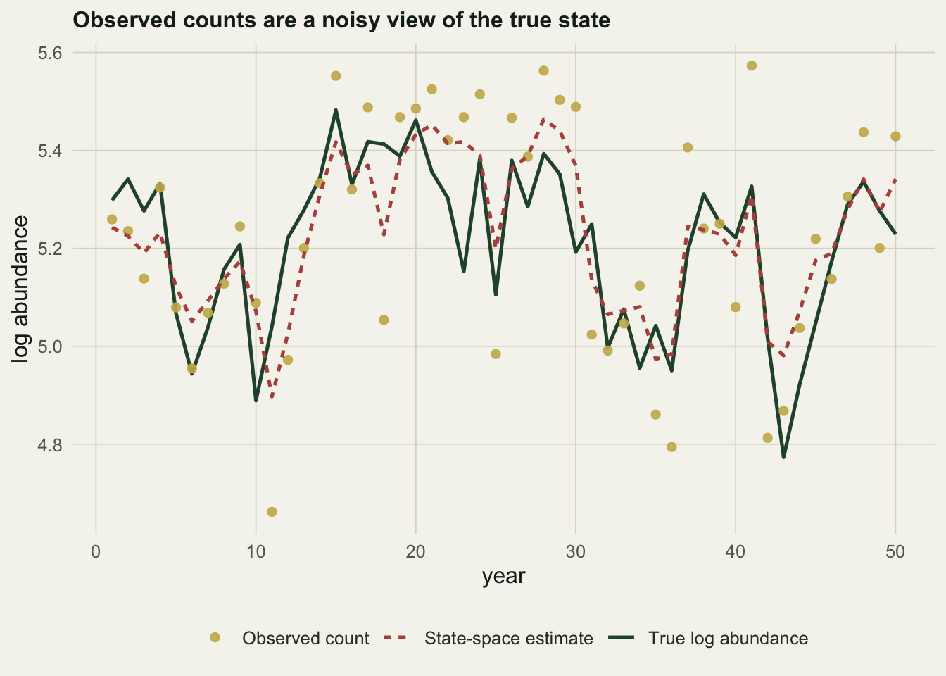
The naive slope comes out at $0.36$, below the true value of $0.70$: taken at face value, the counts overstate how tightly the population is regulated. On this series the state-space model gives $\hat b = 0.59$, closer to the truth, and it splits the variability into a process standard deviation of $0.144$ and an observation standard deviation of $0.144$, both close to the true $0.15$. In the plot that follows, the state-space estimate of the hidden trajectory tracks the true abundance through the observation noise.
```{r}
#| label: fig-observed
#| fig-cap: "The hidden log abundance, the noisy observed counts, and the state-space estimate of the hidden state from the fitted model."
#| fig-alt: "Time series plot showing a solid, jagged true log-abundance line, scattered observed count points around it, and a dashed state-space estimate tracking the true line."
xs <- kf_smooth(Yobs, f$a, f$b, f$sp^2, f$so^2)
d1 <- data.frame(year=1:Tlen, true=Xstate, obs=Yobs, smooth=xs)
ggplot(d1, aes(year))+
  geom_line(aes(y=true, colour="True log abundance"), linewidth=.9)+
  geom_point(aes(y=obs, colour="Observed count"), size=1.8, alpha=.9)+
  geom_line(aes(y=smooth, colour="State-space estimate"), linewidth=.9, linetype="22")+
  scale_colour_manual(values=c("True log abundance"=forest,"Observed count"=gold,"State-space estimate"=aban))+
  labs(x="year", y="log abundance", colour=NULL,
       title="Observed counts are a noisy view of the true state")+
  theme_te()
```
## Does it remove the bias?
One series is an anecdote. To see the average behaviour, generate four hundred series from the same model and compare the naive slope with the state-space slope across all of them.
```{r}
#| label: mc
#| warning: false
set.seed(7100); M<-400; nbv<-numeric(M); gbv<-numeric(M); cv<-integer(M)
for(i in 1:M){ x<-numeric(Tlen); x[1]<-Xstar
  for(t in 1:(Tlen-1)) x[t+1]<-a_true+b_true*x[t]+rnorm(1,0,sp_true)
  y<-x+rnorm(Tlen,0,so_true); nbv[i]<-naive_b(y); ff<-fit_gss(y); gbv[i]<-ff$b; cv[i]<-ff$conv }
round(c(naive_mean=mean(nbv), gss_mean=mean(gbv[cv==0]),
        gss_sd=sd(gbv[cv==0])), 3)
```
The naive slope averages $0.39$, a downward bias of about $0.32$; the state-space slope averages $0.55$, a bias of about $0.15$. Accounting for observation error roughly halves the bias, which is the payoff the model is designed for. It does not remove the bias entirely at this series length, and the spread across series is wide (a standard deviation of about $0.23$), so a single estimate should be read as approximate.
## Why the split is hard
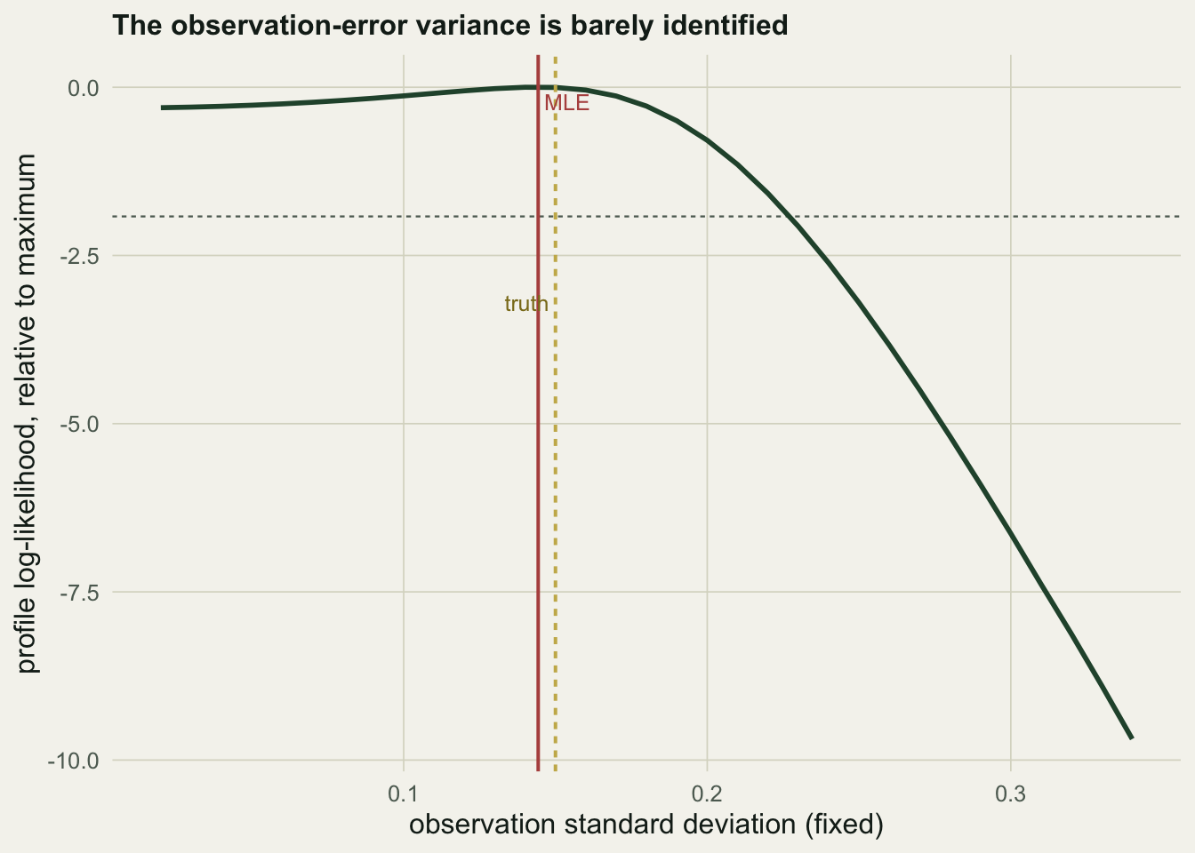
The residual bias and the wide spread are not a coding problem; they are a property of the model. The strength of density dependence and the two variances are only weakly separable from a single series. Fixing the observation variance at a grid of values and re-optimising the rest traces the profile likelihood, and it is nearly flat over a wide range.
```{r}
#| label: profile
so_grid <- seq(0.02, 0.34, by=0.01)
prof <- sapply(so_grid, function(so){
  st<-c(f$a, atanh(min(max(nb,-0.9),0.9)), log(0.02))
  op<-optim(st, kf_nll, y=Yobs, fixed_so2=so^2, method="BFGS", control=list(maxit=1000))
  -op$value })
prof_rel <- prof - max(prof)
range(so_grid[prof_rel > -1.92])   # observation SD values within a 95% likelihood interval
```
Any observation standard deviation between about $0.02$ and $0.22$ sits within a likelihood interval of the maximum. The width of that band is the finding rather than its endpoints, which move with the series and need not reach down to zero: wherever it sits, it stays wide enough that counting error and process error are hard to tell apart. What the likelihood does constrain is their combination, and the fitted total standard deviation is $0.204$ against a true $0.212$. The whole is pinned down; the partition is not.
```{r}
#| label: fig-profile
#| fig-cap: "Profile log-likelihood for the observation standard deviation. The curve is flat across a wide range, so the split between process and observation error is only weakly identified."
#| fig-alt: "Profile log-likelihood curve against observation standard deviation, nearly flat over a wide span of the axis, with the maximum likelihood estimate and the true value marked."
d2 <- data.frame(so=so_grid, rel=prof_rel)
ggplot(d2, aes(so, rel))+
  geom_hline(yintercept=-1.92, colour=faint, linetype="22", linewidth=.4)+
  geom_line(colour=forest, linewidth=1)+
  geom_vline(xintercept=f$so, colour=aban, linewidth=.7)+
  geom_vline(xintercept=so_true, colour=gold, linewidth=.7, linetype="22")+
  annotate("text", x=f$so, y=0, label="MLE ", hjust=1, vjust=1.4, colour=aban, size=3.3)+
  annotate("text", x=so_true, y=-3.2, label=" truth", hjust=0, colour="#8a7a1e", size=3.3)+
  labs(x="observation standard deviation (fixed)", y="profile log-likelihood, relative to maximum",
       title="The observation-error variance is barely identified")+
  theme_te()
```
This weak identifiability, described by Knape, is why the confidence interval for the slope on the single series runs from $-0.15$ to $0.91$: the model is confident there is some density dependence but cannot say how strong, because that answer depends on a variance split the data cannot resolve. The practical advice follows directly. Use the state-space model to avoid the gross bias of ignoring observation error, but do not over-read the individual variance components from a short series, and where an independent estimate of counting error exists, fix the observation variance rather than trying to estimate it. Once density dependence and its measurement are in hand, the natural next question is simply which way the population is heading, which is the subject of [estimating a population trend](../population-trend-estimation/).
## References
Dennis B, Ponciano JM, Lele SR, Taper ML, Staples DF 2006 Ecological Monographs 76(3):323-341 (10.1890/0012-9615(2006)76[323:EDDPNA]2.0.CO;2)
Knape J 2008 Ecology 89(11):2994-3000 (10.1890/08-0071.1)
de Valpine P, Hastings A 2002 Ecological Monographs 72(1):57-76 (10.1890/0012-9615(2002)072[0057:FPMIPN]2.0.CO;2)
Bulmer MG 1975 Biometrics 31(4):901-911 (10.2307/2529815)
## Related tutorials
- [Detecting density dependence](../detecting-density-dependence/)
- [Observation error estimated as zero in a Gompertz fit](../observation-error-estimated-as-zero/)
- [The theta-logistic model](../theta-logistic-model/)
- [Particle MCMC for state space models](../particle-mcmc-for-state-space-models/)