library(ggplot2)

te_paper  <- "#f5f4ee"
te_ink    <- "#16241d"
te_body   <- "#2c3a31"
te_forest <- "#275139"
te_rust   <- "#b5534e"
te_gold   <- "#c9b458"
te_line   <- "#dad9ca"

theme_datasheet <- function() {
  theme_minimal(base_size = 12) +
    theme(plot.background  = element_rect(fill = te_paper, colour = NA),
          panel.background = element_rect(fill = te_paper, colour = NA),
          panel.grid.major = element_line(colour = te_line, linewidth = 0.3),
          panel.grid.minor = element_blank(),
          text             = element_text(colour = te_body),
          plot.title       = element_text(colour = te_ink, face = "bold"),
          plot.subtitle    = element_text(colour = te_body),
          axis.text        = element_text(colour = te_body))
}Particle MCMC for state space models
R
Bayesian statistics
MCMC
state-space models
particle filter
population dynamics
ecology tutorial
A particle filter’s likelihood estimate is noisy but unbiased, so Metropolis-Hastings built on it samples the exact posterior. A Gompertz count model, in R.
A colony of a ground nesting seabird has been counted every season for sixty years. Nobody believes the counts are exact: some burrows are missed, some are counted twice, and in a wet season the survey team works faster. What the ecologist wants to know is how strongly the colony is regulated and how large its real year to year swings are, and both questions are about a population that is never observed directly. A state space model separates the two layers, a hidden log abundance that follows density dependent dynamics and a count that scatters around it. The likelihood of such a model is an integral over every possible hidden path, and for most observation models that integral has no closed form.
This post fits that kind of model by particle marginal Metropolis-Hastings, the method Andrieu, Doucet and Holenstein set out in 2010. The idea is short enough to state in one sentence: run a particle filter at each proposed parameter value, use its likelihood estimate in place of the true likelihood in an ordinary Metropolis-Hastings ratio, and keep the estimate attached to the current state until a proposal is accepted. The claim that makes it worth learning is stronger than the idea. Because the filter’s estimate of the likelihood (not of the log likelihood) is unbiased, the chain has the exact posterior as its stationary distribution, whatever the number of particles. The particle number decides how well the chain mixes, not what it converges to.
Several neighbours on this site cover the pieces. The Gompertz state-space model writes the linear Gaussian version of this model and maximises its likelihood with a hand coded Kalman filter; that filter comes back here as the gold standard, because for that one observation model the likelihood is exact. A particle filter for animal movement builds a bootstrap filter by hand and runs it with the movement parameters held at their true values, so it estimates tracks rather than parameters. This post puts a filter of the same kind inside a sampler that estimates the parameters. ABC-MCMC and sequential ABC samplers is the useful contrast: those samplers replace the likelihood with a tolerance on summary statistics, and that post says plainly that its three samplers target the same approximate posterior. Particle MCMC replaces the likelihood with a random but unbiased estimate of it, and the posterior it targets is not approximate at all.
That claim is testable, so the post tests it. A two parameter Gompertz model with lognormal counting error has an exact likelihood from the Kalman filter and a posterior computed on a fine grid, exact up to quadrature error. Particle chains with three different particle numbers are compared with that posterior, using Monte Carlo standard errors built from effective sample sizes. A tempting variant that re-estimates the current state’s likelihood at every iteration is run alongside them, and it is not exact. The last section moves to Poisson counts, where no Kalman filter exists, and uses the standard deviation of the log likelihood estimate to choose the particle number before the real run.
A count series with an exact answer
The hidden state is the log abundance. It reverts towards an equilibrium at a rate set by the density dependence coefficient b, and it is pushed around by process noise with standard deviation sigma. Writing the equilibrium as mu makes this the Gompertz model of the neighbouring post with its intercept equal to mu times one minus b. The first count uses the stationary distribution of the process, so no starting value has to be invented. The observed log count adds independent normal error with standard deviation tau.
To keep the exact posterior computable on a grid, two quantities are treated as known: the equilibrium log abundance and the counting error, as if the second came from a survey with repeated counts. The unknowns are b and the log of sigma. The prior is uniform on b between minus one and one, which is the stationary region, and normal on log sigma with mean log 0.5 and standard deviation one.
n_t      <- 60
mu_log   <- log(50)
b_true   <- 0.7
sig_true <- 0.3
tau_obs  <- 0.3

set.seed(2108)
x_true    <- numeric(n_t)
x_true[1] <- rnorm(1, mu_log, sig_true / sqrt(1 - b_true^2))
for (i in 2:n_t) {
  x_true[i] <- mu_log + b_true * (x_true[i - 1] - mu_log) + rnorm(1, 0, sig_true)
}
y_log   <- x_true + rnorm(n_t, 0, tau_obs)
y_count <- rpois(n_t, exp(x_true))

log_prior <- function(b, lsig) {
  ifelse(abs(b) < 1, dnorm(lsig, log(0.5), 1, log = TRUE), -Inf)
}

# exact log likelihood by the Kalman filter, vectorised over parameter values
kalman_ll <- function(b, sig, y = y_log) {
  a_m <- rep(mu_log, length(b))
  p_v <- sig^2 / (1 - b^2)
  ll  <- 0
  for (i in seq_along(y)) {
    if (i > 1) {
      a_m <- mu_log + b * (a_m - mu_log)
      p_v <- b^2 * p_v + sig^2
    }
    f_v <- p_v + tau_obs^2
    v_i <- y[i] - a_m
    ll  <- ll - 0.5 * (log(2 * pi * f_v) + v_i^2 / f_v)
    a_m <- a_m + p_v / f_v * v_i
    p_v <- p_v - p_v^2 / f_v
  }
  ll
}

b_grid  <- seq(-0.995, 0.995, by = 0.005)
ls_grid <- seq(log(0.03), log(1.5), length.out = 300)
post_grid <- expand.grid(b = b_grid, lsig = ls_grid)
lp_grid   <- kalman_ll(post_grid$b, exp(post_grid$lsig)) +
  log_prior(post_grid$b, post_grid$lsig)
post_grid$w <- exp(lp_grid - max(lp_grid))
post_grid$w <- post_grid$w / sum(post_grid$w)

ex_mean <- c(b = sum(post_grid$w * post_grid$b),
             lsig = sum(post_grid$w * post_grid$lsig))
ex_cov  <- cov.wt(as.matrix(post_grid[, c("b", "lsig")]), post_grid$w,
                  method = "ML")$cov
ex_sd   <- sqrt(diag(ex_cov))
ex_cor  <- ex_cov[1, 2] / prod(ex_sd)
edge_mass <- sum(post_grid$w[abs(post_grid$b) > 0.98 |
                             post_grid$lsig < log(0.05) |
                             post_grid$lsig > log(1.2)])
n_grid_pts <- nrow(post_grid)
For a linear Gaussian model the Kalman filter is not an approximation: it computes the likelihood exactly, as a product of one step ahead predictive densities. Evaluated on a grid of 119700 parameter pairs, it gives the posterior to within quadrature error. The posterior mean of b is 0.6238 with a posterior standard deviation of 0.1451, and the posterior mean of log sigma is -1.3290 with a standard deviation of 0.2016; the two are correlated at -0.42. The grid is wide enough: the posterior mass in its outer margins is 3.86e-04. Those four numbers are what every sampler below has to reproduce.
The filter’s likelihood is unbiased on the right scale
The bootstrap filter is the one the movement post builds, with two changes that matter for the likelihood estimate: particles start from the stationary distribution, and they are resampled multinomially at every step rather than systematically when the effective sample size drops. At every count the particles are weighted by the observation density. The mean weight at each step estimates the predictive density of that count, and the product of those means over the sixty steps estimates the likelihood. Resampling happens before the particles are pushed through the process model. Andrieu, Doucet and Holenstein define the estimator exactly this way, and it is unbiased for the likelihood for any particle number of one or more.
Two implementation choices matter for speed. Many filters are run at once, laid end to end in one long vector, so that one call can evaluate the likelihood for every chain in a sampler. And the weights are handled on the log scale, with each filter’s largest log weight subtracted before exponentiating, which is added back exactly so the estimate is unchanged.
# bootstrap particle filter for many parameter values at once;
# n_part[k] particles for filter k, laid end to end in one vector
pf_loglik <- function(b, sig, n_part, y, obs, log_mean = FALSE) {
  n_f   <- length(b)
  n_all <- sum(n_part)
  blk   <- rep(seq_len(n_f), n_part)
  off   <- blk - 1
  b_end <- cumsum(n_part)
  bb    <- b[blk]
  ss    <- sig[blk]
  xp    <- mu_log + rnorm(n_all) * ss / sqrt(1 - bb^2)
  ll    <- numeric(n_f)
  ll_logmean <- numeric(n_f)
  for (i in seq_along(y)) {
    if (i > 1) {
      # multinomial resampling inside each filter, then propagate
      cw  <- cumsum(w_norm)
      cw  <- pmin(cw - c(0, cw[b_end][-n_f])[blk], 1) + off
      cw[b_end] <- seq_len(n_f)
      anc <- findInterval(off + runif(n_all), cw, left.open = TRUE) + 1
      xp  <- mu_log + bb * (xp[anc] - mu_log) + ss * rnorm(n_all)
    }
    lw <- if (obs == "lognormal") {
      dnorm(y[i], xp, tau_obs, log = TRUE)
    } else {
      dpois(y[i], exp(xp), log = TRUE)
    }
    lw  <- pmax(lw, -1e5)
    m_f <- cummax(lw + off * 1e6)[b_end] - (seq_len(n_f) - 1) * 1e6
    wt  <- exp(lw - m_f[blk])
    s_f <- diff(c(0, cumsum(wt)[b_end]))
    # log of the MEAN weight: the unbiased factor for this step
    ll  <- ll + m_f + log(s_f / n_part)
    if (log_mean) {
      ll_logmean <- ll_logmean + diff(c(0, cumsum(lw)[b_end])) / n_part
    }
    w_norm <- wt / s_f[blk]
  }
  if (log_mean) list(ll = ll, ll_logmean = ll_logmean) else ll
}

ll_at_mean <- kalman_ll(ex_mean[1], exp(ex_mean[2]))
n_rep_ub   <- 4000
n_part_ub  <- 50

set.seed(311)
ub_run <- pf_loglik(rep(ex_mean[1], n_rep_ub), rep(exp(ex_mean[2]), n_rep_ub),
                    rep(n_part_ub, n_rep_ub), y_log, "lognormal", log_mean = TRUE)
log_err   <- ub_run$ll - ll_at_mean
ratio_ub  <- exp(log_err)
ratio_mean <- mean(ratio_ub)
ratio_se   <- sd(ratio_ub) / sqrt(n_rep_ub)
ratio_z    <- (ratio_mean - 1) / ratio_se
log_bias   <- mean(log_err)
log_sd     <- sd(log_err)
half_var   <- -log_sd^2 / 2
logmean_bias <- mean(ub_run$ll_logmean - ll_at_mean)
share_below  <- mean(ratio_ub < 1)

n_part_big <- 500
n_rep_big  <- 50
ub_big <- pf_loglik(rep(ex_mean[1], n_rep_big), rep(exp(ex_mean[2]), n_rep_big),
                    rep(n_part_big, n_rep_big), y_log, "lognormal", log_mean = TRUE)
logmean_bias_big <- mean(ub_big$ll_logmean - ll_at_mean)
log_bias_big     <- mean(ub_big$ll - ll_at_mean)
The check is direct. At the exact posterior mean the filter was run 4000 times with 50 particles, and each estimate was divided by the exact Kalman likelihood. The mean of that ratio is 0.991 with a Monte Carlo standard error of 0.026, which puts it 0.33 standard errors from one.
The same runs on the log scale tell a different story. The mean error of the log likelihood estimate is -0.738, with a standard deviation of 1.255. That bias is not a flaw in the filter: a positive estimate with mean one and a log that is roughly normal must have a log mean near minus half the log variance, which here is -0.788. The typical estimate is too small, 71.8 per cent of them fall below the true likelihood, and a few large ones restore the mean. Averaging on the log scale is the wrong thing to do with this estimator.
A filter that averages the log weights instead of the weights shows how wrong. That is what mean(log(w)) computes where log(mean(w)) belongs. Its log likelihood error on the same runs averages -36.20, and with 500 particles it still averages -35.88, because the mean of the log weights converges to a different quantity from the log of the mean weight, and more particles only make it converge there faster. The correct estimator at 500 particles has a mean log error of 0.002.
ub_df <- data.frame(log_err = log_err)
ggplot(ub_df, aes(log_err)) +
  geom_histogram(bins = 60, fill = te_line, colour = NA) +
  geom_vline(xintercept = 0, colour = te_forest, linewidth = 0.9) +
  geom_vline(xintercept = log_bias, colour = te_rust, linewidth = 0.9,
             linetype = "dashed") +
  labs(x = "estimated minus exact log likelihood", y = "filter runs",
       title = "Mostly too low, right on average",
       subtitle = paste0("green: exact; dashed red: mean log error ",
                         sprintf("%.2f", log_bias),
                         "; mean likelihood ratio ",
                         sprintf("%.3f", ratio_mean))) +
  theme_datasheet()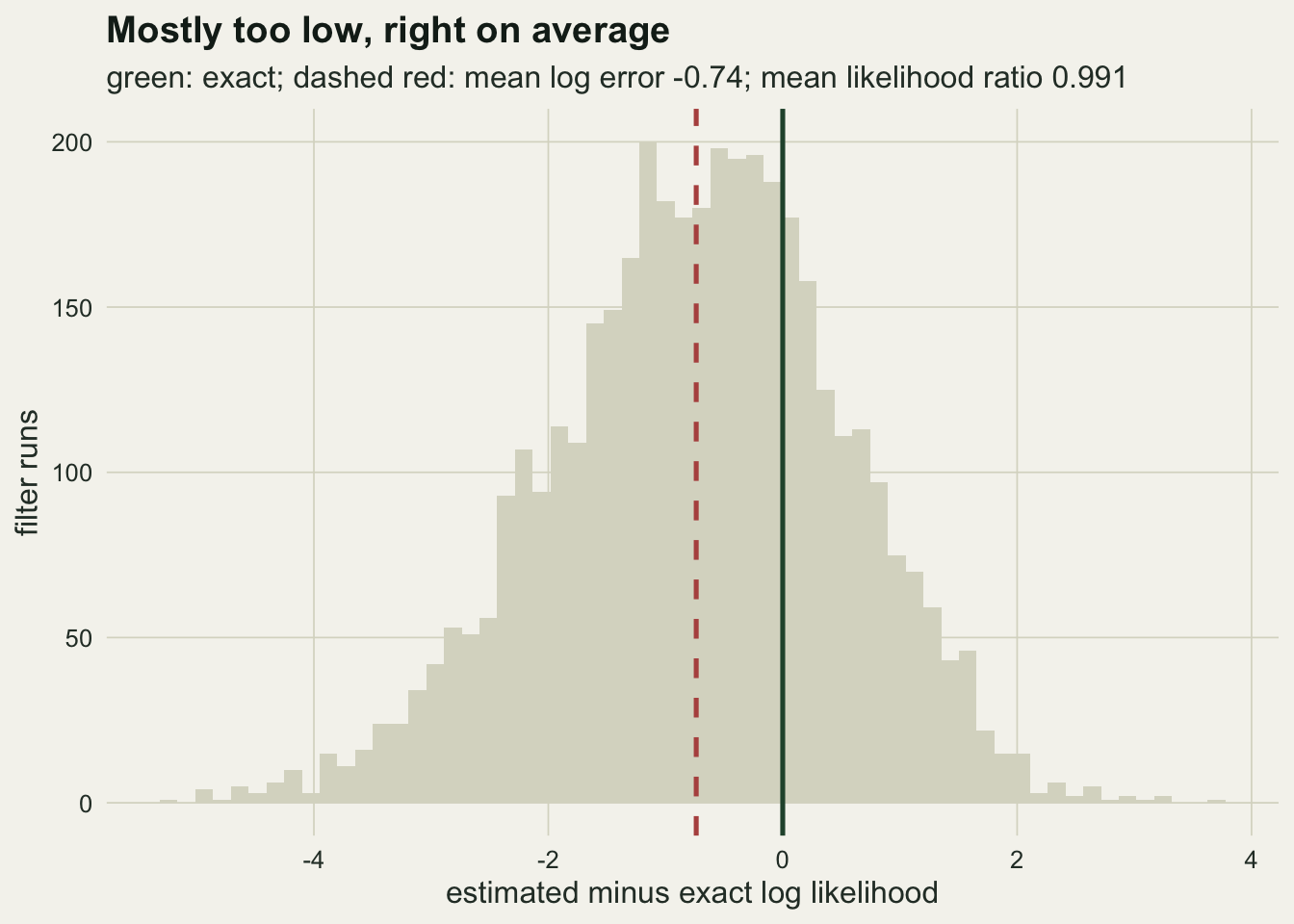
Pseudo-marginal Metropolis-Hastings
The sampler is a random walk Metropolis-Hastings chain on b and log sigma in which the exact likelihood is replaced by the filter’s estimate. Andrieu and Roberts called this the pseudo-marginal approach and gave the reason it works. Think of the random numbers inside the filter as an extra variable. The chain then samples a joint distribution of parameters and filter noise, in which the likelihood estimate plays the part of the likelihood. Because the estimate has mean equal to the true likelihood, integrating the filter noise out leaves the exact posterior as the marginal for the parameters.
One detail carries all the weight. The likelihood estimate for the current state must be the one computed when that state was accepted, and it must stay attached to it until the next acceptance. The code below keeps it in ll_cur and only overwrites it when a proposal is taken.
n_iter   <- 3000
n_burn   <- 750
n_chain  <- 4
The particle numbers were fixed from a pilot study of the standard deviation of the log likelihood estimate at the exact posterior mean, run before any chain: ten particles give a standard deviation near three, fifty give a value near the practical guideline of 1.2 discussed below, and two hundred and fifty give about half. Every chain uses the same proposal, a normal random walk with covariance 2.38 squared over two times the exact posterior covariance, so that acceptance rates differ only because of the likelihood noise. Four chains per setting start from the same scattered values; each runs 3000 iterations and the first 750 are discarded.
# effective sample size across chains (a Geyer-style initial positive sequence),
# as in the convergence diagnostics post
ess_geyer <- function(draws) {
  n_it <- nrow(draws)
  n_ch <- ncol(draws)
  w_in <- mean(apply(draws, 2, var))
  b_bt <- n_it * var(colMeans(draws))
  v_plus <- ((n_it - 1) / n_it) * w_in + b_bt / n_it
  acov <- sapply(seq_len(n_ch), function(j) {
    acf(draws[, j], lag.max = n_it - 1, type = "covariance", plot = FALSE)$acf
  })
  rho <- 1 - (w_in - rowMeans(acov)[-1]) / v_plus
  tau_int <- 1
  k <- 1
  while (k + 1 <= length(rho)) {
    pair <- rho[k] + rho[k + 1]
    if (pair < 0) break
    tau_int <- tau_int + 2 * pair
    k <- k + 2
  }
  c(ess = n_ch * n_it / tau_int, rhat = sqrt(v_plus / w_in))
}
pmmh_run <- function(n_iter, init, n_part, refresh, loglik, prop_cov) {
n_c <- nrow(init)
theta <- init
chol_p <- chol(prop_cov)
ll_cur <- loglik(theta, n_part)
lp_cur <- log_prior(theta[, 1], theta[, 2])
keep_b <- keep_ls <- matrix(NA_real_, n_iter, n_c)
n_acc <- numeric(n_c)
ref <- which(refresh)
for (it in seq_len(n_iter)) {
theta_new <- theta + matrix(rnorm(2 * n_c), n_c, 2) %*% chol_p
lp_new <- log_prior(theta_new[, 1], theta_new[, 2])
theta_eval <- theta_new
theta_eval[!is.finite(lp_new), 1] <- 0
# one call: proposals for every chain, plus a fresh estimate at the
# current state for the refreshing (wrong) chains only
ll_all <- loglik(rbind(theta_eval, theta[ref, , drop = FALSE]),
c(n_part, n_part[ref]))
ll_new <- ll_all[seq_len(n_c)]
if (length(ref) > 0) ll_cur[ref] <- ll_all[n_c + seq_along(ref)]
take <- log(runif(n_c)) < ll_new + lp_new - ll_cur - lp_cur
theta[take, ] <- theta_new[take, ]
ll_cur[take] <- ll_new[take]
lp_cur[take] <- lp_new[take]
n_acc <- n_acc + take
keep_b[it, ] <- theta[, 1]
keep_ls[it, ] <- theta[, 2]
}
list(b = keep_b, lsig = keep_ls, acc = n_acc / n_iter)
}
init_one <- cbind(c(0.2, 0.9, 0.5, 0.8), log(c(0.15, 0.6, 0.4, 0.2)))
prop_cov <- 2.38^2 / 2 * ex_cov
cfg <- data.frame(
label = c("exact likelihood", "N = 10", "N = 50", "N = 250",
"refreshed, N = 10", "refreshed, N = 50"),
n_part = c(0, 10, 50, 250, 10, 50),
refresh = c(FALSE, FALSE, FALSE, FALSE, TRUE, TRUE))
pf_cfg <- cfg[-1, ]
set.seed(5923)
run_exact <- pmmh_run(n_iter, init_one, rep(0, n_chain), rep(FALSE, n_chain),
function(th, np) kalman_ll(th[, 1], exp(th[, 2])),
prop_cov)
run_pf <- pmmh_run(n_iter, init_one[rep(seq_len(n_chain), nrow(pf_cfg)), ],
rep(pf_cfg$n_part, each = n_chain),
rep(pf_cfg$refresh, each = n_chain),
function(th, np) pf_loglik(th[, 1], exp(th[, 2]), np,
y_log, "lognormal"),
prop_cov)chain_summary <- function(kb, ks, acc, lab, cost) {
kb <- kb[-seq_len(n_burn), , drop = FALSE]
ks <- ks[-seq_len(n_burn), , drop = FALSE]
e_b <- ess_geyer(kb)
e_ls <- ess_geyer(ks)
data.frame(label = lab, acc = mean(acc),
mean_b = mean(kb), mcse_b = sd(kb) / sqrt(e_b[1]), sd_b = sd(kb),
ess_b = e_b[1], rhat_b = e_b[2],
mean_ls = mean(ks), mcse_ls = sd(ks) / sqrt(e_ls[1]),
sd_ls = sd(ks), ess_ls = e_ls[1], rhat_ls = e_ls[2],
cost = cost, row.names = NULL)
}
tab <- chain_summary(run_exact$b, run_exact$lsig, run_exact$acc, cfg$label[1], NA)
for (k in seq_len(nrow(pf_cfg))) {
cols <- (k - 1) * n_chain + seq_len(n_chain)
tab <- rbind(tab, chain_summary(run_pf$b[, cols], run_pf$lsig[, cols],
run_pf$acc[cols], pf_cfg$label[k],
pf_cfg$n_part[k] * (1 + pf_cfg$refresh[k])))
}
tab$z_b <- (tab$mean_b - ex_mean[1]) / tab$mcse_b
tab$z_ls <- (tab$mean_ls - ex_mean[2]) / tab$mcse_ls
n_kept <- n_chain * (n_iter - n_burn)
tab$ess_min <- pmin(tab$ess_b, tab$ess_ls)
# effective draws per million particle propagations
tab$ess_rate <- tab$ess_min / (tab$cost * n_kept * n_t) * 1e6
set.seed(8817)
n_rep_sd <- 100
n_grid_part <- c(5, 10, 20, 50, 100, 250, 500, 1000)
sd_ln <- vapply(n_grid_part, function(np) {
sd(pf_loglik(rep(ex_mean[1], n_rep_sd), rep(exp(ex_mean[2]), n_rep_sd),
rep(np, n_rep_sd), y_log, "lognormal"))
}, numeric(1))
sd_at <- function(np) sd_ln[n_grid_part == np]
r_ex <- tab[1, ]; r10 <- tab[2, ]; r50 <- tab[3, ]; r250 <- tab[4, ]
rf10 <- tab[5, ]; rf50 <- tab[6, ]
z_max_pm <- max(abs(c(tab$z_b[2:4], tab$z_ls[2:4])))
rate_ratio_250 <- r50$ess_rate / r250$ess_rateThe data frame tab holds the result. With the exact likelihood the chain accepts 0.351 of its proposals. With particle estimates the acceptance rate is 0.027 at ten particles, 0.200 at fifty and 0.302 at two hundred and fifty. Measured again at the exact posterior mean, with 100 filter runs per particle number, the standard deviations of the log likelihood estimate at those three particle numbers were 2.95, 1.14 and 0.55; at fifty particles the 4000 runs of the first section give the better estimate, 1.26.
No particle chain is far from the exact posterior means. For b the three particle chains give 0.6408, 0.6207 and 0.6157 against the exact 0.6238, with Monte Carlo standard errors of 0.0331, 0.0068 and 0.0055. For log sigma they give -1.3583, -1.3279 and -1.3237 against -1.3290. The largest discrepancy across the six comparisons is 1.45 standard errors, but the standard error at ten particles is 4.9 times the one at fifty, so that setting is the least tested. Each standard error is the posterior standard deviation over the square root of the effective sample size, not of the number of draws.
What changes is the effective sample size. From 9000 kept draws, the chain at ten particles yields 8 effective draws for its worse parameter, the chain at fifty yields 500, the chain at two hundred and fifty 770, and the exact chain 1119. The largest R-hat at ten particles is 1.154, which is a sign that the chains are too short for that setting, and a standard error resting on 8 effective draws is not a check of anything.
So the ten particle setting was run again, after the result above had been seen, with sixteen chains instead of four (the four starting values each used four times, and a new seed), and nothing else changed. The extra chains are cheap, because ten particles cost little and all the chains share one filter call per iteration.
n_chain_big <- 16
set.seed(7741)
run_10big <- pmmh_run(n_iter, init_one[rep(seq_len(n_chain), 4), ],
                      rep(10, n_chain_big), rep(FALSE, n_chain_big),
                      function(th, np) pf_loglik(th[, 1], exp(th[, 2]), np,
                                                 y_log, "lognormal"),
                      prop_cov)
r10big <- chain_summary(run_10big$b, run_10big$lsig, run_10big$acc,
                        "N = 10, 16 chains", 10)
r10big$z_b  <- (r10big$mean_b - ex_mean[1]) / r10big$mcse_b
r10big$z_ls <- (r10big$mean_ls - ex_mean[2]) / r10big$mcse_ls
r10big$ess_min  <- min(r10big$ess_b, r10big$ess_ls)
r10big$ess_rate <- r10big$ess_min /
  (10 * n_chain_big * (n_iter - n_burn) * n_t) * 1e6
rate_ratio_10big <- r50$ess_rate / r10big$ess_rate
With sixteen chains the ten particle setting gives 205 effective draws for its worse parameter and a largest R-hat of 1.035. Its posterior mean of b is 0.6372 with a standard error of 0.0099, 1.36 standard errors from the exact value, and its mean of log sigma is -1.3197, 0.83 standard errors away. Its acceptance rate is 0.038.
trace_df <- do.call(rbind, lapply(1:3, function(k) {
  col_k <- (k - 1) * n_chain + 1
  keep  <- (n_burn + 1):n_iter
  data.frame(iter = keep, b = run_pf$b[keep, col_k],
             setting = pf_cfg$label[k])
}))
trace_df$setting <- factor(trace_df$setting, levels = pf_cfg$label[1:3])
ggplot(trace_df, aes(iter, b)) +
  geom_hline(yintercept = ex_mean[1], colour = te_rust, linewidth = 0.6,
             linetype = "dashed") +
  geom_line(colour = te_forest, linewidth = 0.35) +
  facet_wrap(~ setting, ncol = 1) +
  labs(x = "iteration", y = "b",
       title = "Few particles make a sticky chain",
       subtitle = "dashed red: exact posterior mean of b") +
  theme_datasheet() +
  theme(strip.text = element_text(colour = te_ink, face = "bold"))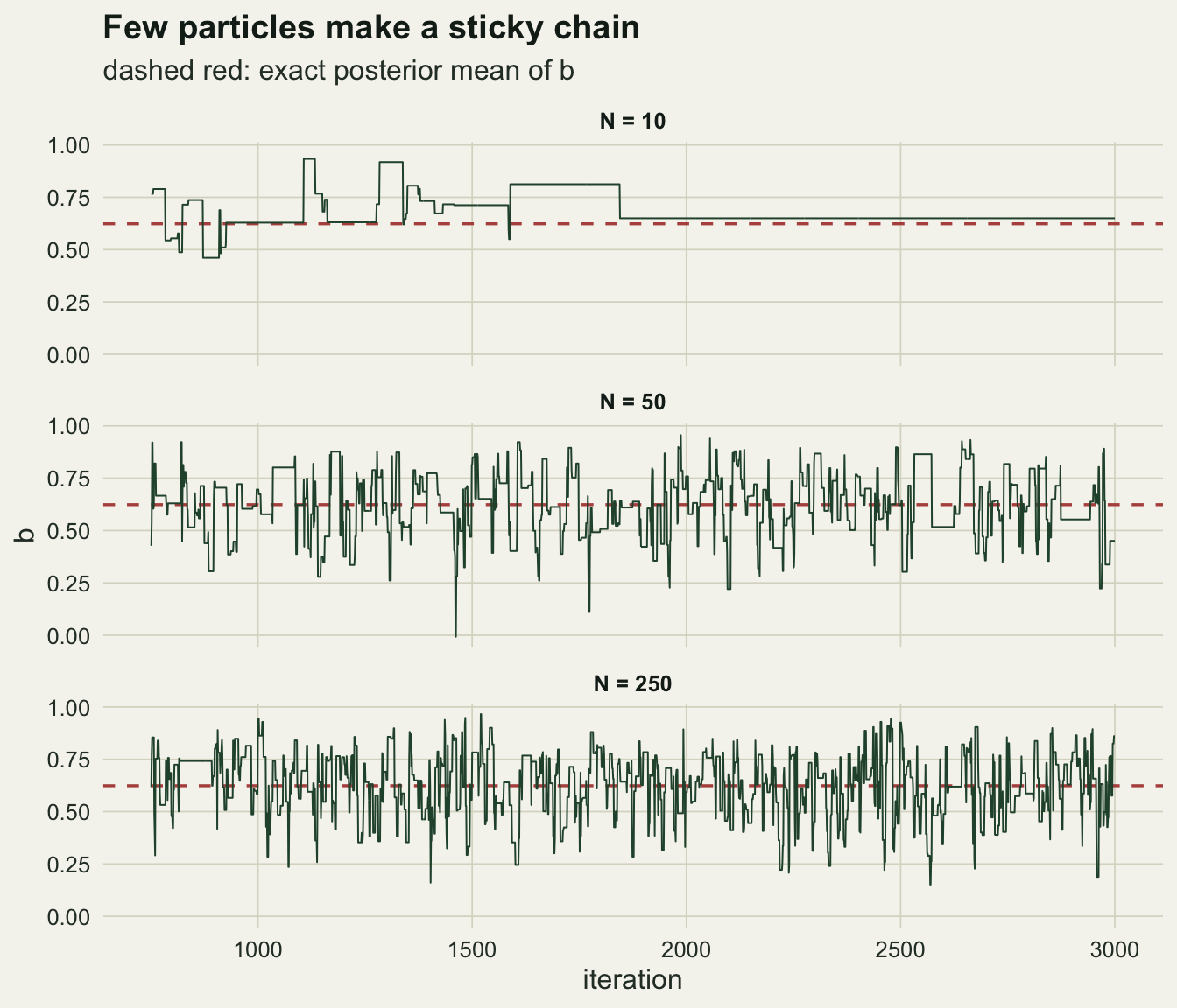
Cost is the other half of the choice. A filter with more particles costs more to run, so the fair comparison is effective draws per unit of work. Counting work as particle propagations, the chain at fifty particles delivers 18.5 effective draws per million, against 9.5 at ten (from the sixteen chain run, whose effective sample size is the less unreliable of the two) and 5.7 at two hundred and fifty. That makes fifty particles 1.9 times as efficient as ten and 3.2 times as efficient as two hundred and fifty. Each ratio rests on one run per setting, so treat the factor against ten particles as rough. Doucet, Pitt, Deligiannidis and Kohn derived the optimum under a Gaussian noise assumption: the standard deviation of the log likelihood estimate should sit near one when the proposal would be efficient with the exact likelihood and near 1.7 when it would not, and they suggest about 1.2 in practice. With a perfect proposal, drawing straight from the posterior, their optimum falls to 0.92. Of the three particle numbers run here, the one closest to that guideline is also the most efficient.
Refreshing the current estimate is not exact
The sticky chain at ten particles invites a fix. A chain sticks because one estimate at the current state came out lucky and high, and no proposal can beat it. So estimate the current state’s likelihood afresh at every iteration, and compare two fresh estimates. This is the Monte Carlo within Metropolis scheme that Andrieu and Roberts analyse next to the pseudo-marginal chain, and they state that the posterior is typically not its invariant distribution, so it does not sample the posterior even in steady state. The code above runs it by passing refresh = TRUE, which costs a second filter run per iteration.
dens_b <- function(v) {
  d_k <- density(v, from = -0.2, to = 1, n = 512)
  data.frame(b = d_k$x, dens = d_k$y)
}
marg_exact <- aggregate(w ~ b, data = post_grid, FUN = sum)
marg_exact$dens <- marg_exact$w / 0.005
col_50  <- (2 - 1) * n_chain + seq_len(n_chain)   # second setting: N = 50
col_r10 <- (4 - 1) * n_chain + seq_len(n_chain)   # fourth setting: refreshed, N = 10
keep    <- (n_burn + 1):n_iter
dens_df <- rbind(
  data.frame(dens_b(c(run_pf$b[keep, col_50])), setting = "pseudo-marginal, N = 50"),
  data.frame(dens_b(c(run_pf$b[keep, col_r10])), setting = "refreshed, N = 10"))
sd_ratio_r10 <- rf10$sd_b / ex_sd[1]
sd_ratio_r50 <- rf50$sd_b / ex_sd[1]
The refreshed chains mix easily, and that is the trap. At ten particles the refreshed chain accepts 0.410 of its proposals and gives 433 effective draws of b. Its posterior mean for b is 0.5259 with a standard error of 0.0129, which is 7.6 standard errors below the exact 0.6238, and its posterior standard deviation for b is 0.268, 1.85 times the exact value. At fifty particles the error is smaller but still resolved: a mean of 0.5992, 4.2 standard errors away, and a standard deviation 1.26 times the exact one.
Both refreshed chains are too wide, and both are pulled towards smaller b, which in this model means stronger density dependence. With two fresh noisy estimates in every ratio, a proposal into a poorly fitting region is sometimes accepted on luck, and the chain has no memory that would correct it later. The error shrinks with more particles, but at fifty it was still resolved, and nothing in the chain’s own diagnostics reveals it: the R-hat of the refreshed chain at ten particles is 1.004.
Is the problem that the filter is noisier in some parts of the parameter space than in others? A control answers that. The same refreshed scheme is run with the exact Kalman log likelihood plus fresh normal noise whose standard deviation is the same everywhere, set to the measured value at ten particles and to the better estimate at fifty, with mean minus half the variance so that the likelihood stays unbiased.
set.seed(2917)
n_chain_ctl <- 16
ctl_noise <- c(sd_at(10), log_sd)
ctl <- do.call(rbind, lapply(ctl_noise, function(s_n) {
  run_c <- pmmh_run(n_iter, init_one[rep(seq_len(n_chain), 4), ],
                    rep(0, n_chain_ctl), rep(TRUE, n_chain_ctl),
                    function(th, np) kalman_ll(th[, 1], exp(th[, 2])) +
                      rnorm(nrow(th), -s_n^2 / 2, s_n),
                    prop_cov)
  kb <- run_c$b[-seq_len(n_burn), ]
  data.frame(noise_sd = s_n, mean_b = mean(kb), sd_ratio = sd(kb) / ex_sd[1])
}))
With constant noise of standard deviation 2.95 the refreshed chain gives a mean for b of 0.555 and a posterior standard deviation 1.87 times the exact one, against 0.526 and 1.85 with the particle filter at ten particles. With noise of 1.26 it gives 0.607 and 1.30, against 0.599 and 1.26 at fifty particles. Constant noise of the same size reproduces the widening and most of the shift in the mean, so the distortion does not need noise that varies over the parameter space.
ggplot() +
  geom_area(data = marg_exact[marg_exact$b >= -0.2, ], aes(b, dens),
            fill = te_line, colour = NA) +
  geom_line(data = dens_df, aes(b, dens, colour = setting), linewidth = 1) +
  scale_colour_manual(values = c(te_forest, te_rust), name = NULL) +
  labs(x = "density dependence coefficient b", y = "posterior density",
       title = "Keep the estimate, and the posterior is exact",
       subtitle = "grey area: exact posterior from the Kalman likelihood on a grid") +
  theme_datasheet() +
  theme(legend.position = "bottom")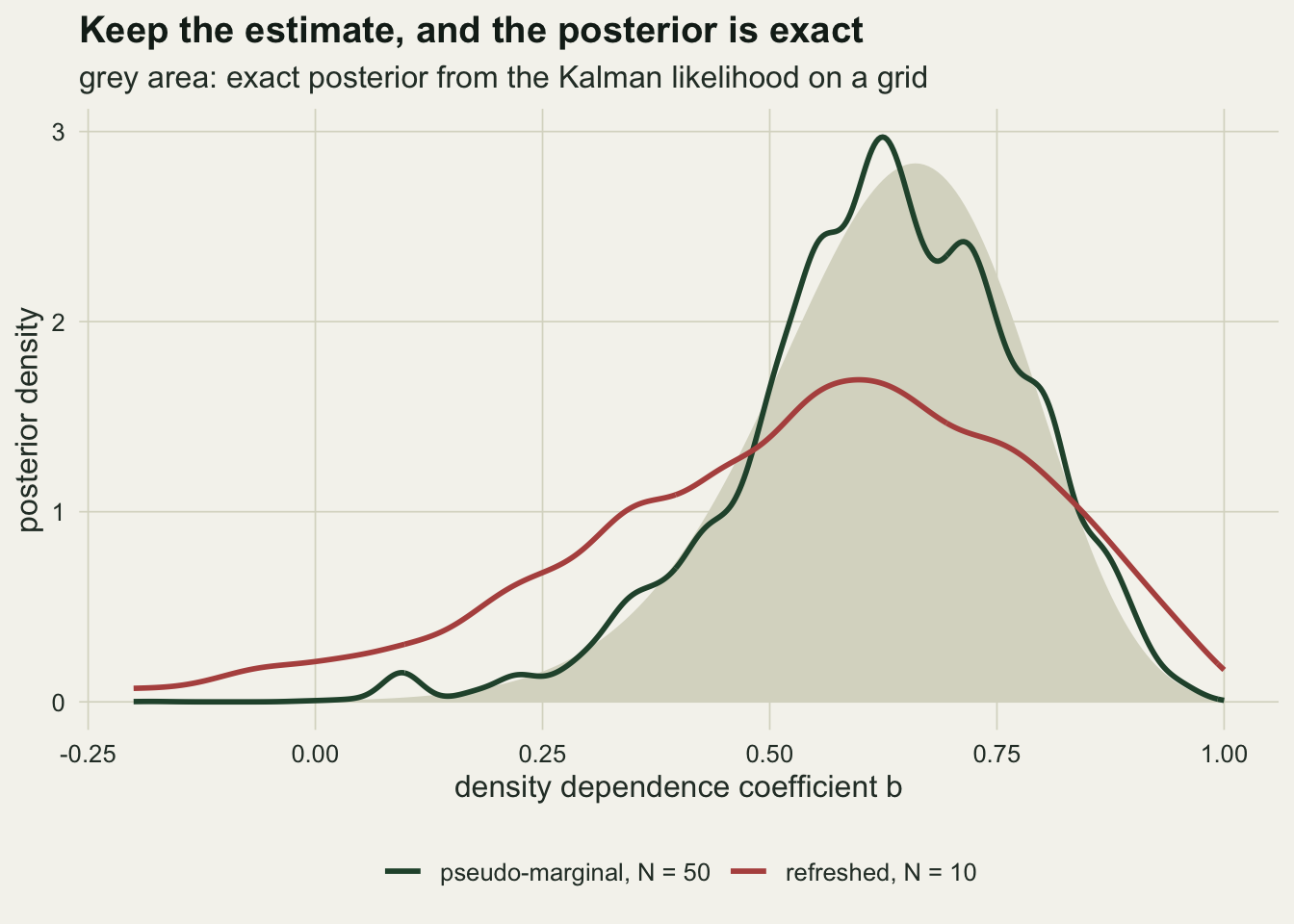
tab_fig <- rbind(tab, r10big[, names(tab)])
fig_levels <- c(cfg$label[1:2], r10big$label, cfg$label[3:6])
mean_df <- rbind(
  data.frame(label = tab_fig$label, param = "b", est = tab_fig$mean_b,
             mcse = tab_fig$mcse_b, exact = unname(ex_mean[1])),
  data.frame(label = tab_fig$label, param = "log sigma", est = tab_fig$mean_ls,
             mcse = tab_fig$mcse_ls, exact = unname(ex_mean[2])))
mean_df$label <- factor(mean_df$label, levels = rev(fig_levels))
mean_df$kind  <- ifelse(grepl("refreshed", mean_df$label), "refreshed (wrong)",
                        "exact or pseudo-marginal")
ggplot(mean_df, aes(est, label, colour = kind)) +
  geom_vline(aes(xintercept = exact), colour = te_body, linetype = "dashed",
             linewidth = 0.5) +
  geom_errorbar(aes(xmin = est - 2 * mcse, xmax = est + 2 * mcse), orientation = "y",
                width = 0.25, linewidth = 0.7) +
  geom_point(size = 2.4) +
  facet_wrap(~ param, scales = "free_x") +
  scale_colour_manual(values = c(te_forest, te_rust), name = NULL) +
  labs(x = "posterior mean", y = NULL,
       title = "Particle number moves the error bar, not the answer") +
  theme_datasheet() +
  theme(legend.position = "bottom",
        strip.text = element_text(colour = te_ink, face = "bold"))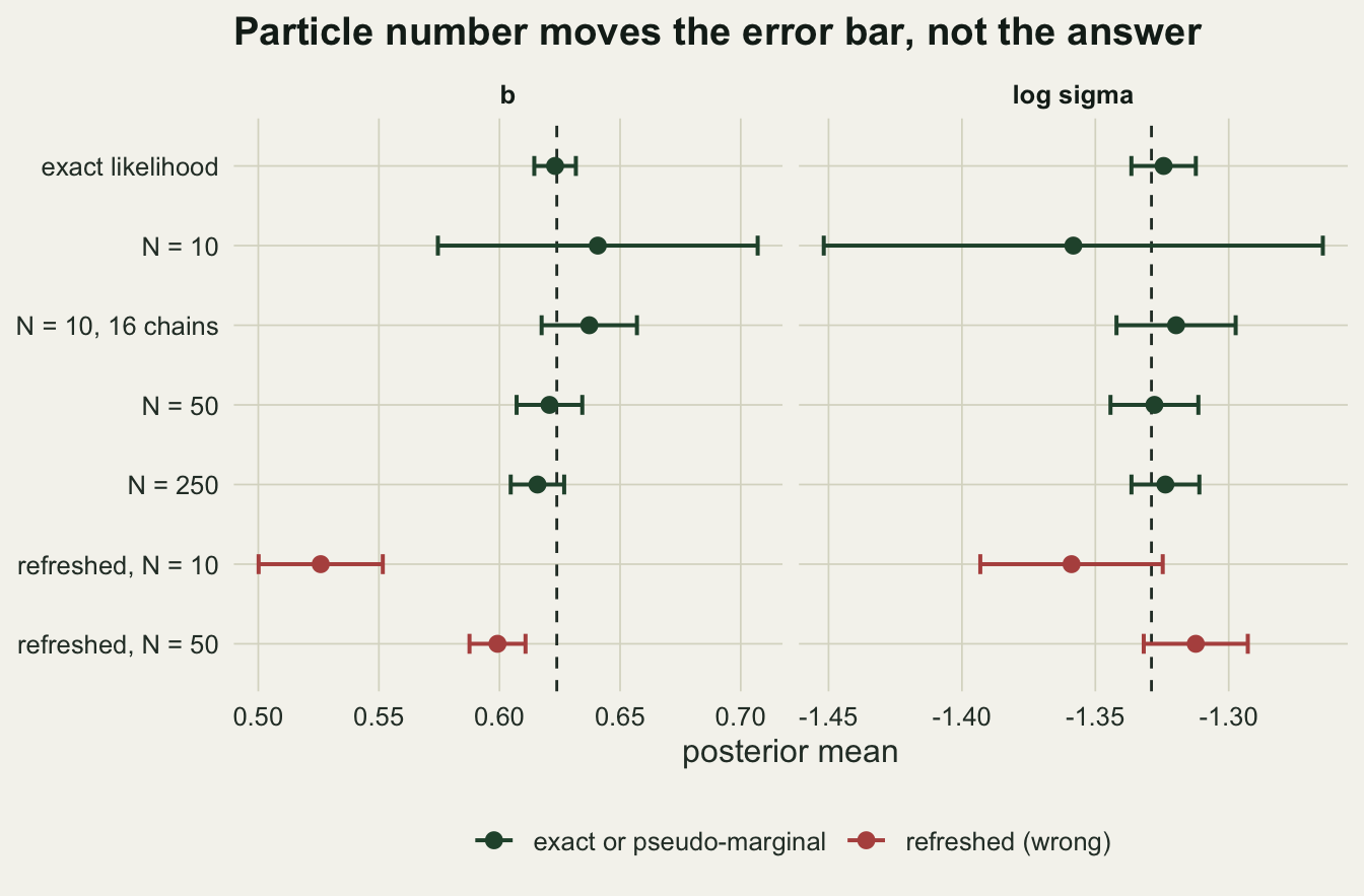
Poisson counts, where no Kalman filter exists
Real colony counts are integers, and a Poisson observation model on the same hidden log abundance is closer to how a count is made. With it there is no Kalman filter and no grid posterior, so the exactness check above is all the assurance there is: the filter changes one line, and the argument does not depend on the observation model.
What does change is the particle number needed. A Poisson count with a mean near fifty has a coefficient of variation of about one in seven, which on the log scale is a tighter observation than the lognormal error of 0.3 used above, and a tighter observation means more peaked weights and a noisier estimate. So the particle number is chosen by the rule rather than copied. A short pilot chain with a hundred particles and a hand set proposal gives a rough posterior mean and covariance; the standard deviation of the log likelihood estimate is measured at that mean over the same grid of particle numbers; and the main run uses the smallest grid value whose standard deviation is at most 1.2. The rule was fixed before the pilot ran.
set.seed(6630)
pilot <- pmmh_run(600, init_one, rep(100, n_chain), rep(FALSE, n_chain),
                  function(th, np) pf_loglik(th[, 1], exp(th[, 2]), np,
                                             y_count, "poisson"),
                  diag(c(0.08, 0.12)^2))
pil_keep   <- 201:600
pilot_draw <- cbind(c(pilot$b[pil_keep, ]), c(pilot$lsig[pil_keep, ]))
pilot_mean <- colMeans(pilot_draw)
pilot_cov  <- cov(pilot_draw)

sd_po <- vapply(n_grid_part, function(np) {
  sd(pf_loglik(rep(pilot_mean[1], n_rep_sd), rep(exp(pilot_mean[2]), n_rep_sd),
               rep(np, n_rep_sd), y_count, "poisson"))
}, numeric(1))
sd_target <- 1.2
n_sel     <- n_grid_part[which(sd_po <= sd_target)[1]]
sd_sel    <- sd_po[n_grid_part == n_sel]
n_ln_sel  <- n_grid_part[which(sd_ln <= sd_target)[1]]
sd_po_50  <- sd_po[n_grid_part == 50]

n_iter_po <- 2000
n_burn_po <- 500
run_po <- pmmh_run(n_iter_po, init_one, rep(n_sel, n_chain), rep(FALSE, n_chain),
                   function(th, np) pf_loglik(th[, 1], exp(th[, 2]), np,
                                              y_count, "poisson"),
                   2.38^2 / 2 * pilot_cov)
n_burn_keep <- n_burn
n_burn <- n_burn_po
po_tab <- chain_summary(run_po$b, run_po$lsig, run_po$acc, "Poisson", n_sel)
n_burn <- n_burn_keep
po_sig <- exp(po_tab$mean_ls)
po_sd_ratio <- po_tab$sd_b / ex_sd[1]

# Monte Carlo error of a standard deviation from n_rep_sd runs, from the
# kurtosis of the 4000 lognormal log errors (no new random numbers)
kurt_err  <- mean((log_err - log_bias)^4) / mean((log_err - log_bias)^2)^2
sd_se_100 <- sd_target * sqrt((kurt_err - 1) / (4 * n_rep_sd))

# better estimates at the decision points, drawn after every chain has run
set.seed(4417)
n_rep_chk <- 1000
sd_po_100_chk <- sd(pf_loglik(rep(pilot_mean[1], n_rep_chk),
                              rep(exp(pilot_mean[2]), n_rep_chk),
                              rep(100, n_rep_chk), y_count, "poisson"))
sd_ln_100_chk <- sd(pf_loglik(rep(ex_mean[1], n_rep_chk), rep(exp(ex_mean[2]), n_rep_chk),
                              rep(100, n_rep_chk), y_log, "lognormal"))
sd_ln_chk <- c(sd_ln[n_grid_part < 50], log_sd, sd_ln_100_chk, sd_ln[n_grid_part > 100])
n_ln_sel_chk <- n_grid_part[which(sd_ln_chk <= sd_target)[1]]
The pilot put the posterior mean of b at 0.729. At that value the standard deviation of the Poisson log likelihood estimate is 1.80 with fifty particles, against 1.26 for the lognormal model at its own posterior mean (from the first section’s runs), and the rule selects 250 particles for the counts, since a hundred give 1.23 and narrowly miss the threshold; at 250 the standard deviation is 0.77. Both decisions sit inside their own Monte Carlo error: with 100 runs, a standard deviation near 1.2 is itself uncertain by about 0.09. A check with 1000 runs gives 1.29 for the counts at a hundred particles, so the choice of 250 stands. For the lognormal model the curve’s 100 runs would select 50, while the 4000 runs at fifty particles in the first section give 1.26, above the threshold, and the 1000 run check gives 0.84 at a hundred; with those better estimates the rule selects 100. The fifty particle chains above were not chosen by this rule, and they were not rerun.
The main run of 2000 iterations per chain accepts 0.266 of its proposals and gives 535 effective draws for its worse parameter, with R-hat values of 1.009 and 1.001. The posterior mean of b is 0.729 with a Monte Carlo standard error of 0.0041 and a posterior standard deviation of 0.096; the posterior mean of log sigma corresponds to a process standard deviation of 0.292. The simulation used b equal to 0.7 and sigma equal to 0.3. The posterior for b is 0.66 times as wide as under the lognormal error model. The two data sets share the hidden series but not the counting error, and Poisson counts near fifty are the more precise of the two, so the narrower posterior is a property of the data rather than of the sampler.
sd_df <- rbind(data.frame(n_part = n_grid_part, sd_ll = sd_ln,
                          model = "lognormal error, tau 0.3"),
               data.frame(n_part = n_grid_part, sd_ll = sd_po,
                          model = "Poisson counts"))
ggplot(sd_df, aes(n_part, sd_ll, colour = model)) +
  annotate("rect", xmin = 4, xmax = 1250, ymin = 1, ymax = 1.7,
           fill = te_gold, alpha = 0.25) +
  geom_hline(yintercept = sd_target, colour = te_body, linetype = "dashed",
             linewidth = 0.5) +
  geom_line(linewidth = 0.9) +
  geom_point(size = 2.2) +
  scale_x_log10(breaks = n_grid_part) +
  scale_y_log10() +
  scale_colour_manual(values = c("lognormal error, tau 0.3" = te_forest,
                                 "Poisson counts" = te_rust), name = NULL) +
  labs(x = "particles (log scale)", y = "sd of log likelihood estimate (log scale)",
       title = "Counts need more particles",
       subtitle = "gold band: 1 to 1.7; dashed: the 1.2 used to choose N") +
  theme_datasheet() +
  theme(legend.position = "bottom")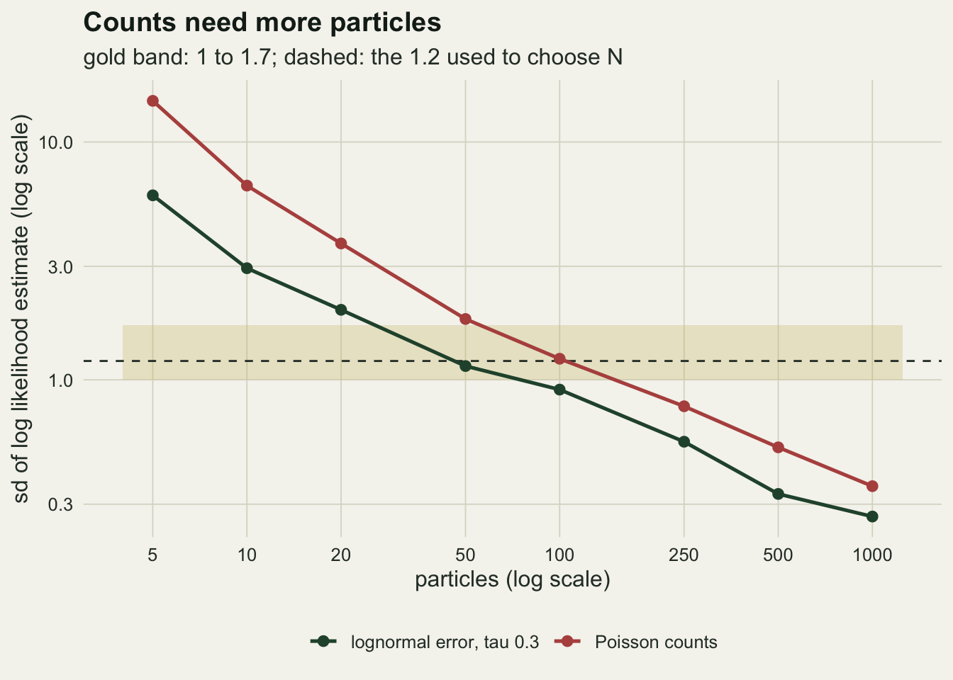
What to report
Report the particle number together with the standard deviation of the log likelihood estimate it gave, and the parameter value where that standard deviation was measured. The particle number alone means nothing outside the data set: the same fifty particles gave 1.26 on one observation model and 1.80 on the other, for the same hidden series.
Report Monte Carlo standard errors from effective sample sizes, and read them before reading the decimals. A pseudo-marginal chain with too few particles is not biased, but its effective sample size can be a small fraction of its length, and here the chain at ten particles kept 8 effective draws out of 9000. The error bar is the honest summary of that.
State that the likelihood estimate at the current state was kept and not refreshed, in words, because that is the line of code on which exactness depends and a reader cannot see it in a posterior table. If a refreshed scheme was used for speed, call it an approximation and say what was done to check it.
Say what the filter’s estimate is: the product over time of the mean weights, with resampling at every step. Adaptive resampling and other estimators can also be unbiased, but a reader should not have to guess.
Honest limits
Only two parameters were estimated. The equilibrium and the counting error were held at their true values so that the exact posterior could be computed on a grid, and in a real analysis both would be unknown. With both variances free, the neighbouring Gompertz post shows that process error and counting error are only weakly separable from a single series, and a random walk proposal tuned on a well behaved two dimensional posterior says little about that case.
The exactness check has limited power. The agreement was measured on posterior means only, from chains of 3000 iterations, and a bias smaller than about two standard errors would not have been detected. On the b scale that is 0.014 at fifty particles and 0.020 for the sixteen chain run at ten. The ten particle setting also needed a second run with more chains, decided after the first had been seen; that run changed the number of chains and the seed and nothing else, and because its effective sample size comes from a few long sticky episodes, its standard errors should be read as rough. The theory does the heavy lifting here; the simulation shows that nothing large went wrong in the code.
The efficiency comparison used three particle numbers and one proposal. It agrees with the guideline, but it cannot locate the optimum, and it counts cost as particle propagations. The fixed overhead of each filter call in R is not proportional to the particle number, so on a clock the smaller filters look worse than they do here.
The refreshed chain was run at two particle numbers on one data set. Its error grows with the noise of the log likelihood estimate, and the control with constant normal noise shows that the distortion does not need noise that varies over the parameter space. The result shows that the scheme is not exact, not how inexact it will be elsewhere.
The Poisson section has no gold standard. Its posterior was checked only for internal consistency across chains, and its particle number came from a pilot mean that was itself estimated with a noisy likelihood.
References
Andrieu C, Doucet A, Holenstein R 2010 Journal of the Royal Statistical Society Series B 72(3):269-342 (10.1111/j.1467-9868.2009.00736.x)
Andrieu C, Roberts GO 2009 The Annals of Statistics 37(2):697-725 (10.1214/07-AOS574)
Doucet A, Pitt MK, Deligiannidis G, Kohn R 2015 Biometrika 102(2):295-313 (10.1093/biomet/asu075)