ABC-MCMC and sequential ABC samplers

Rejection ABC draws from the prior and throws almost all of it away. ABC-MCMC and sequential Monte Carlo recycle the good draws; a Ricker model prices the gain.

Rejection ABC has one obvious flaw: it proposes from the prior forever. It learns nothing. Draw ten thousand parameter vectors, keep the fifty that land near your data, then go back to drawing from the same prior as if the fifty had never happened.

Two families of samplers fix this. ABC-MCMC (Marjoram et al. 2003) walks a chain that lingers where the fit is good. Sequential ABC (Sisson et al. 2007; Beaumont et al. 2009; Toni et al. 2009) carries a population of particles through a ladder of shrinking tolerances, proposing each round from the last round’s survivors.

Both work. Both are worth knowing. But before we write either one, there is a question almost nobody asks: how much is there to win? A sampler can only reallocate simulations towards the good region. If the good region already gets a fair share of the prior’s attention, there is nothing to reallocate. So there is a ceiling, and it is computable from a pilot run in one line, before you write any sampler code at all.

This post builds ABC-MCMC and sequential ABC from scratch, measures both against plain rejection on the same problem, and measures the ceiling. The short version: on this problem the ceiling is about ten, the best sampler delivers about two, and tightening the tolerance does not change that bargain in your favour.

If you have not met rejection ABC, start with rejection ABC from scratch. The model and summaries below come from choosing summary statistics for ABC, so this post reuses that setup without re-deriving it.

The test problem

The Ricker map with environmental noise and Poisson counting error, the standard hard case for likelihood-free inference (Wood 2010). Population n updates multiplicatively, and you observe Poisson counts rather than n itself:

library(ggplot2)

ricker <- function(log_r, sigma, phi = 10, n_time = 100, burn = 50) {
  r <- exp(log_r)
  e <- rnorm(burn + n_time, 0, sigma)
  n <- 1
  out <- numeric(n_time)
  for (t in seq_len(burn + n_time)) {
    n <- r * n * exp(-n + e[t])
    if (t > burn) out[t - burn] <- n
  }
  rpois(n_time, phi * out)
}

Five summaries: the mean count, the number of zeros, and three numbers from a cubic autoregression of y^0.3 on its own lag. The last of those, the residual spread of that regression, is what pins the noise parameter sigma; without it sigma is barely identified.

summ <- function(y) {
  n_time <- length(y)
  z <- y^0.3
  X <- cbind(1, z[-n_time], z[-n_time]^2)
  fit <- tryCatch({
    b <- qr.solve(X, z[-1])
    c(b[2], b[3], sd(z[-1] - X %*% b))
  }, error = function(e) c(0, 0, 0))
  c(mean(y), sum(y == 0), fit[1], fit[2], fit[3])
}

lo <- c(3, 0)
hi <- c(5, 0.8)

The prior is uniform on that box: log r between 3 and 5, sigma between 0 and 0.8. The counting rate phi is treated as known. Simulate one dataset at log r = 3.8, sigma = 0.3, and scale each summary by its prior-predictive median absolute deviation so the distance is not dominated by whichever summary happens to have the largest units:

set.seed(290)
truth <- c(3.8, 0.3)
y_obs <- ricker(truth[1], truth[2])
s_obs <- summ(y_obs)

pilot <- t(replicate(2000, summ(ricker(runif(1, lo[1], hi[1]), runif(1, lo[2], hi[2])))))
sc <- pmax(apply(pilot, 2, mad), 1e-8)

dist_th <- function(th) sqrt(sum(((summ(ricker(th[1], th[2])) - s_obs) / sc)^2))
in_prior <- function(th) all(th >= lo) && all(th <= hi)

The reference: 200,000 draws from the prior

Everything below gets compared against this. Two hundred thousand prior draws, one simulation each, one distance each:

set.seed(2901)
n_ref <- 2e5
th_ref <- cbind(runif(n_ref, lo[1], hi[1]), runif(n_ref, lo[2], hi[2]))
d_ref <- numeric(n_ref)
for (i in seq_len(n_ref)) d_ref[i] <- dist_th(th_ref[i, ])

eps_grid <- c(0.8, 0.5, 0.35, 0.25, 0.2, 0.15)
data.frame(
  eps = eps_grid,
  accept_rate = sapply(eps_grid, function(e) mean(d_ref <= e)),
  sims_per_draw = round(1 / sapply(eps_grid, function(e) mean(d_ref <= e)))
)

   eps accept_rate sims_per_draw
1 0.80    0.096290            10
2 0.50    0.029715            34
3 0.35    0.009485           105
4 0.25    0.002720           368
5 0.20    0.001170           855
6 0.15    0.000275          3636

eps_star <- as.numeric(quantile(d_ref, 0.005))
eps_tight <- as.numeric(quantile(d_ref, 0.001))
rej_rate <- mean(d_ref <= eps_star)
post_ref <- th_ref[d_ref <= eps_star, ]
c(eps_star = eps_star, eps_tight = eps_tight, n_accepted = nrow(post_ref))

    eps_star    eps_tight   n_accepted 
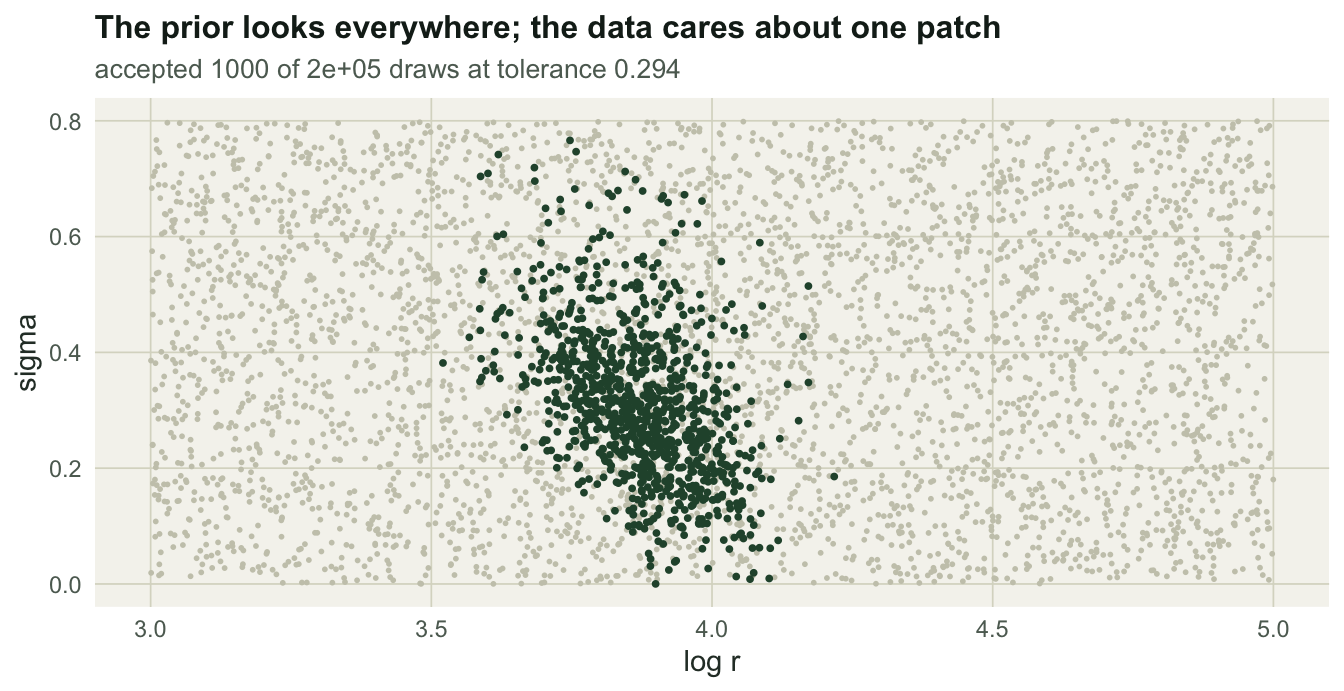
   0.2939077    0.1904299 1000.0000000 

Call eps_star the working tolerance: rejection accepts 0.5 per cent of proposals there, one in 200. That is the number every sampler has to beat.

I will measure everything in effective samples per 1000 simulations. For rejection that is just the acceptance rate: accepted draws are independent, so 5 per 1000. For a chain it is the effective sample size divided by the simulations spent. For a particle population it is the weighted effective sample size divided by the total simulations across all rounds. One currency, three methods.

Figure 1: Where the simulations go. Grey: 4000 of the 200,000 prior draws. Green: every draw accepted at the working tolerance. The prior spreads its effort over the whole box; the accepted draws occupy a small patch of it.

How much is there to win?

Here is the question that decides whether any of this is worth doing.

Let g(theta) be the probability that a simulation run at theta lands within the tolerance. Rejection’s acceptance rate is the average of g over the prior. A perfect sampler, one that already knew the ABC posterior and proposed straight from it, would have an acceptance rate equal to the average of g over the posterior. No sampler can do better, because no sampler can propose from a better distribution than the target itself.

So the ceiling on any sampler’s efficiency gain is the ratio of those two averages. And we can measure it, because we already have a sample from the ABC posterior: the accepted draws. Take an accepted theta, run a fresh simulation at it, and see whether it lands inside the tolerance again. Acceptance was a property of the old simulation; the new one is independent, so this is an unbiased estimate of the posterior average of g.

oracle_rate <- function(eps, n_try, seed) {
  set.seed(seed)
  acc <- th_ref[d_ref <= eps, , drop = FALSE]
  idx <- sample(nrow(acc), n_try, replace = TRUE)
  mean(vapply(seq_len(n_try), function(i) dist_th(acc[idx[i], ]) <= eps, logical(1)))
}

eps_three <- c(eps_star, quantile(d_ref, 0.002), eps_tight)
ceil_tab <- data.frame(
  eps = round(as.numeric(eps_three), 4),
  rejection = sapply(eps_three, function(e) mean(d_ref <= e)),
  oracle = mapply(oracle_rate, eps_three, 15000, c(11, 12, 13))
)
ceil_tab$ceiling <- ceil_tab$oracle / ceil_tab$rejection
ceil_tab

     eps rejection     oracle  ceiling
1 0.2939     0.005 0.05506667 11.01333
2 0.2331     0.002 0.02980000 14.90000
3 0.1904     0.001 0.01146667 11.46667

ceiling_star <- ceil_tab$ceiling[1]
ceiling_star

[1] 11.01333

About 11. That is the entire budget available to cleverness on this problem. Not a factor of a thousand, not an order of magnitude per round: about ten, once, total. Any sampler you write, any sampler anyone has ever written, is fighting over that factor.

Now look down the ceiling column, because this is the part that matters most. Tighten the tolerance from 0.294 to 0.19 and rejection’s acceptance rate falls 5-fold, from one in 200 to one in 1000. The ceiling over the same stretch goes from 11 to 11.5. It does grow, and the theory below says it must: the posterior contracts as the tolerance bites, so the prior looks relatively more wasteful. But it grows by 4 per cent while the bill grows by 400 per cent.

So if your reason for wanting a better sampler is “my tolerance is too loose and I cannot afford to tighten it”, the arithmetic is not on your side. Tightening does hand the sampler slightly more room to work with, and nowhere near enough to pay for itself.

The ceiling, in closed form

You do not have to measure the ceiling with a second round of simulations. If the ABC posterior is roughly Gaussian inside a uniform prior box, the ratio has a closed form. Writing V for the prior volume, p for the number of parameters and S for the ABC posterior covariance:

\[\text{ceiling} \;=\; \frac{V}{(4\pi)^{p/2}\,\sqrt{\det S}}\]

The derivation is short. With a flat prior, the ABC posterior is proportional to g, so rejection’s rate is the integral of g divided by V, while the oracle’s rate is the integral of g squared divided by the integral of g. Put a Gaussian shape into both integrals and the peak height cancels, leaving the expression above. Numerically:

S_post <- cov(post_ref)
ceiling_pred <- prod(hi - lo) / ((4 * pi)^(length(lo) / 2) * sqrt(det(S_post)))
c(predicted = ceiling_pred, measured = ceiling_star)

predicted  measured 
 9.936389 11.013333 

Predicted 9.9, measured 11. One line, one pilot run, no sampler.

Read the formula and the whole business becomes obvious. The ceiling is the prior volume divided by the posterior volume. A sampler’s job is to stop wasting the difference between what you claimed to believe and what the data left you believing. If your prior was already tight, there is no waste, and no sampler helps. If your prior was vague, there is waste in exact proportion to the vagueness.

That last sentence is a testable prediction, so let us test it. Widen the prior on log r from a width of 2 to a width of 6, leaving everything else alone. The formula says the ceiling triples. It also implies something sharper: the extra prior region contributes nothing but wasted simulations, so rejection’s acceptance rate should fall by exactly the same factor of three.

set.seed(2902)
n_wide <- 80000
th_wide <- cbind(runif(n_wide, 1, 7), runif(n_wide, 0, 0.8))
d_wide <- numeric(n_wide)
for (i in seq_len(n_wide)) d_wide[i] <- dist_th(th_wide[i, ])

rate_wide <- mean(d_wide <= eps_star)
c(rate_narrow = rej_rate,
  rate_wide = rate_wide,
  ratio = rej_rate / rate_wide,
  outside_narrow_box = mean(th_wide[d_wide <= eps_star, 1] < 3 | th_wide[d_wide <= eps_star, 1] > 5))

       rate_narrow          rate_wide              ratio outside_narrow_box 
          0.005000           0.001800           2.777778           0.000000 

The acceptance rate falls by a factor of 2.78, against a predicted 3. And of the draws the wide prior did accept, the fraction landing in the region we added is 0. Zero. Two thirds of that budget bought nothing at all, and tripled the ceiling by doing so. A high sampler ceiling is not good news; it is a receipt for a vague prior.

ABC-MCMC

Now the samplers. Marjoram et al. (2003) noticed that you can run Metropolis-Hastings without a likelihood: propose a move, simulate at the proposal, and treat “the simulation landed within the tolerance” as the likelihood evaluation. With a symmetric random-walk proposal and a uniform prior, the Hastings ratio is 1 inside the box and 0 outside, so the whole accept step collapses to two conditions:

abc_mcmc <- function(n_iter, eps, start, step, seed) {
  set.seed(seed)
  out <- matrix(0, n_iter, 2)
  cur <- start
  acc <- 0L
  for (i in seq_len(n_iter)) {
    prop <- cur + rnorm(2, 0, step)
    if (in_prior(prop) && dist_th(prop) <= eps) {
      cur <- prop
      acc <- acc + 1L
    }
    out[i, ] <- cur
  }
  list(draws = out, acc_rate = acc / n_iter)
}

ess <- function(x) {
  n <- length(x)
  a <- acf(x, lag.max = min(n - 1, 3000), plot = FALSE)$acf[-1]
  k <- which(a < 0.05)[1]
  if (is.na(k)) k <- length(a)
  n / (1 + 2 * sum(a[seq_len(max(k - 1, 1))]))
}

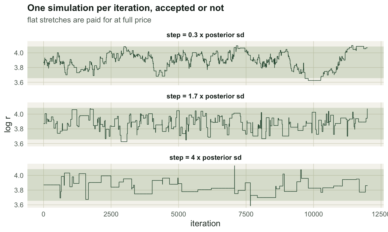
That is the whole algorithm. Ten lines, and one simulation per iteration whether or not the move is accepted, which is the accounting that matters: the cost is n_iter, not the number of accepted moves.

The step size is the only knob, and it is not a cosmetic one. Sweep it from a third of a posterior standard deviation to four:

psd <- apply(post_ref, 2, sd)
m0 <- colMeans(post_ref)
n_it <- 30000

sweep_tab <- do.call(rbind, lapply(c(0.3, 1.0, 1.7, 2.5, 4.0), function(h) {
  M <- abc_mcmc(n_it, eps_star, m0, h * psd, seed = 30 + h * 10)
  keep <- M$draws[-seq_len(3000), ]
  data.frame(step = h,
             acc_rate = M$acc_rate,
             ess_min = min(ess(keep[, 1]), ess(keep[, 2])),
             eff_per_1000 = min(ess(keep[, 1]), ess(keep[, 2])) / n_it * 1000,
             longest_stick = max(rle(keep[, 1])$lengths),
             sd_log_r = sd(keep[, 1]))
}))
sweep_tab

  step   acc_rate    ess_min eff_per_1000 longest_stick   sd_log_r
1  0.3 0.04256667   8.254764    0.2751588          1761 0.11314158
2  1.0 0.03340000  68.138507    2.2712836           541 0.11481595
3  1.7 0.01883333 163.956475    5.4652158           375 0.10455130
4  2.5 0.01160000 119.290308    3.9763436           532 0.10691166
5  4.0 0.00420000  64.762114    2.1587371          1385 0.07437289

best <- sweep_tab[which.max(sweep_tab$eff_per_1000), ]
mcmc_eff <- best$eff_per_1000
worst_eff <- min(sweep_tab$eff_per_1000)
c(best_step = best$step, best_eff = mcmc_eff, worst_eff = worst_eff,
  ratio = mcmc_eff / worst_eff, rejection_eff = rej_rate * 1000)

    best_step      best_eff     worst_eff         ratio rejection_eff 
    1.7000000     5.4652158     0.2751588    19.8620433     5.0000000 

Two things fall out of that table, and the second is the one that will bite you.

First, tuning matters by a factor of 19.9. The best step here is 1.7 posterior standard deviations, which is roughly the textbook random-walk scaling of 2.4 divided by the square root of the dimension. Get it wrong and you are worse than rejection by a wide margin. I got it wrong on my first attempt at this post, chose 0.6, measured ABC-MCMC losing badly to rejection, and nearly wrote that down as a finding.

Second, and worse: look at the sd_log_r column against the rejection reference of 0.108. The badly tuned chains do not merely run slowly. They report a different posterior. The smallest step, the one that shuffles timidly and never covers the target, understates the posterior spread of log r by -5 per cent. That is not a rounding error; it is a credible interval a fifth too narrow, arriving with no warning attached. A chain that spends up to 1761 consecutive iterations at one point has seen a fraction of the target, and the spread it reports is whatever that fraction happened to span. Rejection cannot fail this way. It either accepts a draw or it does not, and the draws it accepts are independent by construction.

Figure 2: Random-walk ABC-MCMC on log r at three step sizes, first 12,000 iterations. The horizontal band is the rejection reference, plus or minus two standard deviations. Flat stretches are rejected proposals: one simulation each, no information.

Now tighten the tolerance and run the tuned chain again:

M_tight <- abc_mcmc(40000, eps_tight, m0, best$step * psd, seed = 77)
k_tight <- M_tight$draws[-seq_len(4000), ]
c(acc_rate = M_tight$acc_rate,
  accepted_moves = round(M_tight$acc_rate * 40000),
  eff_per_1000 = min(ess(k_tight[, 1]), ess(k_tight[, 2])) / 40000 * 1000,
  longest_stick = max(rle(k_tight[, 1])$lengths),
  rejection_eff = mean(d_ref <= eps_tight) * 1000)

      acc_rate accepted_moves   eff_per_1000  longest_stick  rejection_eff 
      0.003975     159.000000       1.273871    1847.000000       1.000000 

Forty thousand simulations bought about 159 accepted moves, the longest stick is 1847 iterations, and the effective yield is now below plain rejection. This is not a tuning failure, and no step size fixes it. The chain’s acceptance probability is g at the proposal, and g is bounded above by the oracle rate, which is exactly the quantity the tolerance is crushing. Tighten the tolerance and the chain’s moves become as rare as rejection’s acceptances, but each effective sample now costs five to ten moves instead of one.

That gives a rule of thumb worth carrying: ABC-MCMC beats rejection only when the ceiling exceeds the chain’s autocorrelation cost, roughly a factor of ten. Here the ceiling is 11. It is a coin flip, and the measurements agree: 5.5 against 5 effective samples per 1000 simulations at the working tolerance.

Sequential ABC

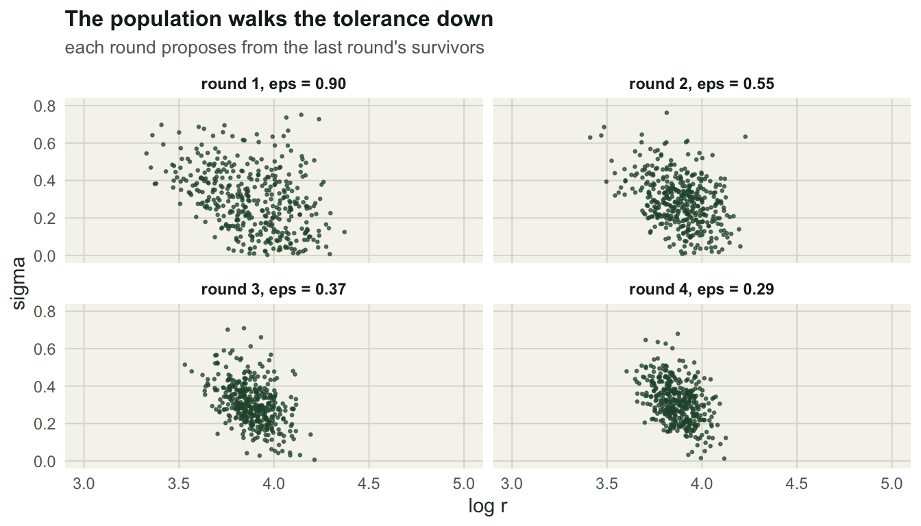
The sequential family attacks the same waste from a different angle. Keep a population of N particles. Round 1 is plain rejection at a generous tolerance. Each later round proposes by picking a surviving particle and jittering it, then shrinks the tolerance to a quantile of the distances the last round achieved. The population walks the tolerance down.

The catch is that particles resampled from round t-1 and jittered are no longer a sample from the prior, so they need importance weights. Sisson et al. (2007) gave the first version of this and it turned out to carry a bias; Beaumont et al. (2009) traced the bias and replaced the correction with a straight importance-sampling weight, which is what I use here. The weight is the prior density divided by the mixture density the proposal actually came from, and the kernel is twice the weighted covariance of the previous population, both taken from that paper.

smc_abc <- function(n_part, alpha, target, eps1 = 0.9, seed) {
  set.seed(seed)
  th <- matrix(0, n_part, 2)
  d <- numeric(n_part)
  w <- rep(1 / n_part, n_part)
  total <- 0L
  eps <- eps1
  round_id <- 0L
  hist <- list()
  clouds <- list()
  repeat {
    round_id <- round_id + 1L
    if (round_id > 1) eps <- max(as.numeric(quantile(d, alpha)), target)
    th_old <- th
    w_old <- w
    tries <- 0L
    if (round_id > 1) L <- chol(2 * cov.wt(th_old, wt = w_old)$cov)
    th_new <- matrix(0, n_part, 2)
    d_new <- numeric(n_part)
    for (i in seq_len(n_part)) {
      repeat {
        tries <- tries + 1L
        p <- if (round_id == 1) {
          c(runif(1, lo[1], hi[1]), runif(1, lo[2], hi[2]))
        } else {
          th_old[sample.int(n_part, 1, prob = w_old), ] + as.numeric(crossprod(L, rnorm(2)))
        }
        if (round_id > 1 && !in_prior(p)) next
        dd <- dist_th(p)
        if (dd <= eps) {
          th_new[i, ] <- p
          d_new[i] <- dd
          break
        }
      }
    }
    if (round_id > 1) {
      dens <- numeric(n_part)
      for (j in seq_len(n_part)) {
        z <- backsolve(L, t(sweep(th_new, 2, th_old[j, ], "-")), transpose = TRUE)
        dens <- dens + w_old[j] * exp(-0.5 * colSums(z^2))
      }
      w <- 1 / dens
      w <- w / sum(w)
    }
    th <- th_new
    d <- d_new
    total <- total + tries
    hist[[round_id]] <- data.frame(round = round_id, eps = eps, sims = tries,
                                   ess = 1 / sum(w^2), cum_sims = total)
    clouds[[round_id]] <- data.frame(round = round_id, eps = eps,
                                     log_r = th[, 1], sigma = th[, 2])
    if (eps <= target + 1e-12 || round_id > 12) break
  }
  list(particles = th, weights = w, total = total, ess = 1 / sum(w^2),
       hist = do.call(rbind, hist), clouds = do.call(rbind, clouds))
}

The prior enters twice and both places matter. A proposal jittered outside the box has prior density zero and must be thrown away before it costs a simulation, which is the next in the inner loop. And the weight is the prior density (constant, hence the bare 1 /) over the proposal mixture density.

Run it to the same working tolerance at three shrink schedules, from aggressive to cautious:

smc_tab <- do.call(rbind, lapply(c(0.3, 0.5, 0.7), function(a) {
  S <- smc_abc(n_part = 400, alpha = a, target = eps_star, seed = 900 + a * 10)
  data.frame(alpha = a, rounds = nrow(S$hist), total_sims = S$total,
             ess = S$ess, eff_per_1000 = S$ess / S$total * 1000)
}))
smc_tab

  alpha rounds total_sims      ess eff_per_1000
1   0.3      4      32933 370.3441    11.245380
2   0.5      6      45493 358.1485     7.872608
3   0.7     10      67600 371.9075     5.501590

best_alpha <- smc_tab$alpha[which.max(smc_tab$eff_per_1000)]
S_main <- smc_abc(n_part = 400, alpha = best_alpha, target = eps_star, seed = 900 + best_alpha * 10)
S_main$hist

  round       eps  sims      ess cum_sims
1     1 0.9000000  2906 400.0000     2906
2     2 0.5505244  4406 367.0021     7312
3     3 0.3722719 10512 372.6869    17824
4     4 0.2939077 15109 370.3441    32933

smc_eff <- max(smc_tab$eff_per_1000)
final_round_rate <- 400 / S_main$hist$sims[nrow(S_main$hist)]
c(smc_eff = smc_eff, final_round_accept = final_round_rate,
  rejection_accept = rej_rate, final_vs_rejection = final_round_rate / rej_rate)

           smc_eff final_round_accept   rejection_accept final_vs_rejection 
       11.24538046         0.02647429         0.00500000         5.29485737 

The schedule matters, and it matters in the direction that costs cautious people money: aggressive shrinking wins by 2 times. Keeping only the best 30 per cent of each round’s distances gets there in 4 rounds; keeping the best 70 per cent takes 10, and every one of those rounds buys a fresh population at full price. The effective sample size at the end is the same to within noise in all three cases, around 367. You do not buy accuracy with a gentle schedule; you buy rounds.

That is the accounting the whole method turns on. Look at the round-by-round table. The final round accepts at 26.5 per 1000, which is 5.3 times rejection’s rate and a respectable fraction of the oracle. Sequential ABC really does learn where to look. But you paid for every earlier round to get there, and those simulations are in the bill: 32,933 in total against 15,109 in the round that did the good work. End to end the gain is 2.2 times, not 5.3.

This is the honest way to report a sequential sampler, and it is not always how it gets reported. A final-round acceptance rate is a real number about a real round. It is not the cost of the answer.

Figure 3: Sequential ABC particle populations at the best-performing schedule. Each panel is one round; the tolerance shrinks left to right. The population walks itself into the posterior, and each round’s proposals are drawn from the previous round’s survivors.

The scoreboard

Same problem, same tolerance, same currency:

board <- data.frame(
  method = c("rejection", "ABC-MCMC (tuned)", "sequential ABC", "oracle (unreachable)"),
  eff_per_1000 = c(rej_rate * 1000, mcmc_eff, smc_eff, ceil_tab$oracle[1] * 1000)
)
board$vs_rejection <- board$eff_per_1000 / (rej_rate * 1000)
board

                method eff_per_1000 vs_rejection
1            rejection     5.000000     1.000000
2     ABC-MCMC (tuned)     5.465216     1.093043
3       sequential ABC    11.245380     2.249076
4 oracle (unreachable)    55.066667    11.013333

rbind(
  rejection = c(colMeans(post_ref), apply(post_ref, 2, sd)),
  abc_mcmc = {
    M <- abc_mcmc(30000, eps_star, m0, best$step * psd, seed = 33)
    k <- M$draws[-seq_len(3000), ]
    c(colMeans(k), apply(k, 2, sd))
  },
  sequential = {
    w <- S_main$weights
    m <- colSums(S_main$particles * w)
    c(m, sqrt(colSums(w * sweep(S_main$particles, 2, m)^2)))
  }
)

               [,1]      [,2]      [,3]      [,4]
rejection  3.870925 0.3129493 0.1075671 0.1325863
abc_mcmc   3.859966 0.3318742 0.1036378 0.1310449
sequential 3.868874 0.3191077 0.1013448 0.1259416

The four columns are the posterior means and standard deviations of log r and sigma. All three samplers agree, which is the point: they are three ways to sample the same approximate posterior, and none of them is more correct than the others. They differ only in price.

Figure 4: Effective samples per 1000 simulations at the working tolerance. The dashed line is the oracle: a sampler that already knew the answer. Everything any sampler can ever win is the gap between the first bar and that line.

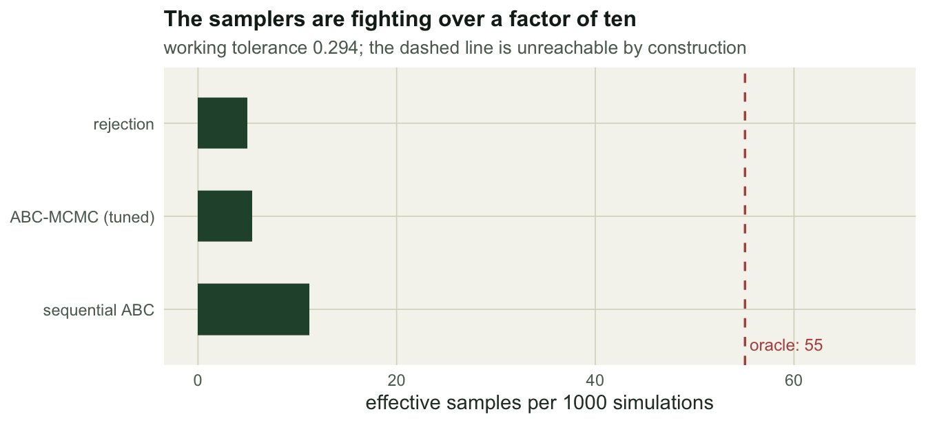
Sequential ABC wins, by about 2.2 times. ABC-MCMC is a wash. The oracle sits at 11 times and cannot be reached. So the best available sampler collects roughly 20 per cent of a prize that was worth ten-fold to begin with.

What this means for your ABC

Compute the ceiling first. It costs one pilot run and one line:

ceiling <- prod(hi - lo) / ((4 * pi)^(length(lo) / 2) * sqrt(det(cov(accepted))))

Then read it:

Ceiling below about 5. Your prior is already close to your posterior. Use rejection, spend the afternoon on something else, and be quietly pleased: a low ceiling means you knew a lot before you started.

Ceiling around 10 to 100. Sequential ABC is worth the fifty lines. ABC-MCMC is a coin flip against rejection and brings a failure mode rejection does not have, namely a stuck chain that reports a confidently wrong posterior. Rejection cannot mislead you that way; it either accepts or it does not.

Ceiling in the thousands. Something is wrong upstream. A prior a thousand times wider than the data’s answer is not a cautious prior, it is a prior you did not think about. Fix that first: the sampler is downstream of it, and no sampler recovers information the prior threw away by being vague in directions the data was going to rule out anyway.

And the case that sends most people looking for a better sampler in the first place: your tolerance is too loose and you cannot afford to tighten it. The ceiling column above is the answer, and the answer is no. Tightening the tolerance shrinks every rate on the scoreboard together, oracle included. Whatever multiple you needed, you still need it after switching samplers.

The things that actually move that particular wall are elsewhere, and this series has visited two of them: better summaries, which shrink the distance without shrinking the tolerance (choosing summary statistics for ABC), and regression adjustment, which corrects the accepted draws for their tolerance-induced spread instead of trying to eliminate it (Beaumont et al. 2002). Wood (2010) goes further still and replaces the tolerance with a Gaussian likelihood fitted to the summaries, which is a different bargain rather than a better sampler.

Honest limits

The ceiling formula assumes a roughly Gaussian ABC posterior inside a uniform prior box. Multimodal posteriors break the derivation, and a heavy-tailed or strongly curved one will bend it. The measured version, which resamples accepted draws and re-simulates, has no such assumption and is what I would trust; the formula is for the back of an envelope.

Two parameters is a friendly case. The ceiling grows roughly like the prior-to-posterior volume ratio raised to the parameter count, so in ten dimensions there is far more for a sampler to win, and sequential ABC earns its keep in a way it does not here. The flip side is that the tolerance is punishing more dimensions of summary space at the same time, so the absolute rates are worse for everyone.

The effective sample sizes for the chains are themselves estimates, and the badly mixing ones are estimated badly. When a chain returns an effective sample size in the tens, treat the number as an indictment rather than a measurement.

And the comparison is per simulation, not per second. Sequential ABC has a per-proposal overhead that rejection does not: a weight calculation that is quadratic in the particle count. When your simulator is a Ricker map, that overhead is visible. When your simulator is an individual-based model that takes a minute per run, it rounds to zero, and per-simulation accounting is the only accounting that matters.

Related tutorials

• Rejection ABC from scratch
• Choosing summary statistics for ABC
• MCMC convergence diagnostics
• Checking an ABC analysis

References

Marjoram P, Molitor J, Plagnol V, Tavare S 2003 Proceedings of the National Academy of Sciences 100(26):15324-15328 (10.1073/pnas.0306899100)

Sisson SA, Fan Y, Tanaka MM 2007 Proceedings of the National Academy of Sciences 104(6):1760-1765 (10.1073/pnas.0607208104)

Beaumont MA, Cornuet JM, Marin JM, Robert CP 2009 Biometrika 96(4):983-990 (10.1093/biomet/asp052)

Toni T, Welch D, Strelkowa N, Ipsen A, Stumpf MPH 2009 Journal of the Royal Society Interface 6(31):187-202 (10.1098/rsif.2008.0172)

Beaumont MA, Zhang W, Balding DJ 2002 Genetics 162(4):2025-2035 (10.1093/genetics/162.4.2025)

Wood SN 2010 Nature 466(7310):1102-1104 (10.1038/nature09319)