Checking an ABC analysis

Three checks for approximate Bayesian computation in ecology: rank calibration for the sampler, posterior width for the answer, acceptance distance for the model.

An ABC posterior always arrives. The usual tolerance rule keeps the closest 0.25 per cent of simulations, so something is always accepted, and the accepted parameters always make a histogram that looks like a posterior. Nothing in the algorithm can refuse.

That leaves three questions which sound alike and are not. Is the sampler returning what it claims to return? Has the analysis learned anything? Can the model produce data like yours at all? This post builds one check for each, on the Ricker benchmark the rest of this cluster uses. Each check is blind to the question the next one asks, and the blindness is not a detail: the standard calibration check passes, at full marks, on an analysis whose intervals cover half of what they promise.

The model, the priors and the summaries

The simulator is the noisy Ricker map with Poisson counts (Wood 2010). A population grows by r, is thinned by its own density, is shaken by process noise of size sigma, and is counted with detection scaled by phi = 10.

sim_ricker <- function(log_r, sigma, T = 50, phi = 10, N0 = 1) {
  M <- length(log_r)
  N <- rep(N0, M)
  Y <- matrix(0L, M, T)
  r <- exp(log_r)
  for (t in seq_len(T)) {
    N <- r * N * exp(-N + rnorm(M, 0, sigma))
    Y[, t] <- rpois(M, phi * N)
  }
  Y
}

summ <- function(Y) {
  n  <- ncol(Y)
  L  <- log1p(Y)
  Lc <- L - rowMeans(L)
  acf1 <- rowSums(Lc[, -1, drop = FALSE] * Lc[, -n, drop = FALSE]) / rowSums(Lc^2)
  S <- cbind(mean  = rowMeans(Y),                # average count
             sdlog = sqrt(rowMeans(Lc^2)),       # spread on the log scale
             acf1  = acf1,                       # year to year autocorrelation
             zeros = rowMeans(Y == 0))           # how often the count is zero
  S[!is.finite(S)] <- 0        # a series pinned at zero has no autocorrelation
  S
}

prior <- function(M) cbind(log_r = runif(M, 3, 5), sigma = runif(M, 0, 0.8))

set.seed(4291)
th_pilot <- prior(20000)
sc       <- apply(summ(sim_ricker(th_pilot[, 1], th_pilot[, 2])), 2, mad)
fit_cols <- names(sc)
round(sc, 3)

 mean sdlog  acf1 zeros 
8.525 0.139 0.147 0.237 

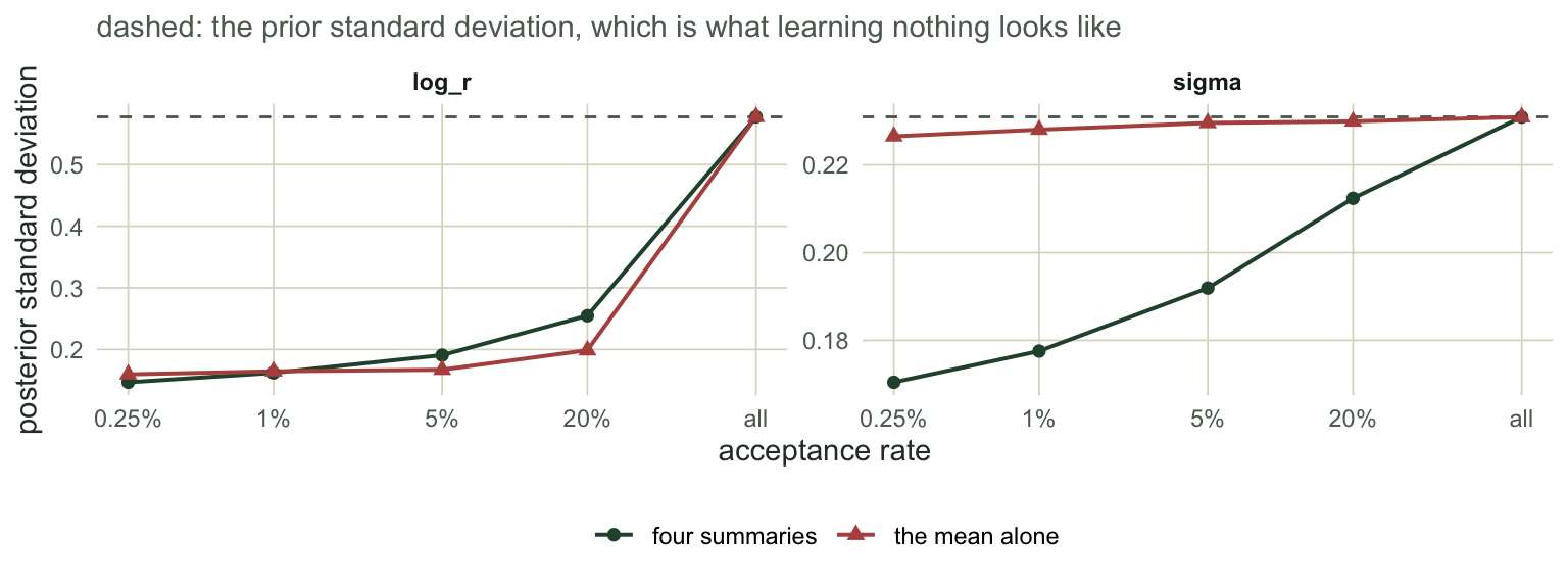
Each summary is divided by its pilot MAD and the distance is Euclidean on that scale. The four are the ones an ecologist reaches for first. The priors are flat on log_r in [3, 5] and on sigma in [0, 0.8], which is the noisy chaotic region where the likelihood is intractable and ABC earns its keep. Note the prior standard deviations that the width of a uniform buys you: 0.577 for log_r and 0.231 for sigma. Any posterior standard deviation near those numbers is a posterior that learned nothing.

Check 1: is the sampler returning what it claims?

The check is older than ABC (Cook, Gelman and Rubin 2006) and has a version written for it (Prangle et al. 2014). Draw a parameter from the prior, simulate a data set from it, run the entire analysis on that data set, and record where the drawn parameter falls among the posterior draws. Repeat. If the posterior is exact, the drawn parameter is itself a draw from it, so its rank among L posterior draws is uniform on 0, 1, ..., L. A rank histogram that is not flat proves the machine is not delivering the posterior it claims.

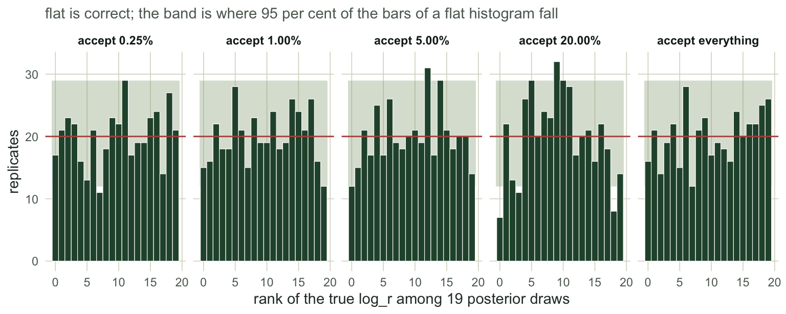
Fix L = 19 so the histograms are comparable across settings, and note the bonus: the truth should fall outside the range of 19 draws twice in twenty by chance, so the range is a 90 per cent interval that costs no quantile estimate.

The tolerance enters as an acceptance rate. Five rates share one reference pool per replicate, so the whole sweep costs one pass. The last rate accepts everything, which is not a mistake; it is the other end of the sweep, and it is the reason this post has a second section.

n_rep <- 400
M     <- 8000
arms  <- c(0.0025, 0.01, 0.05, 0.20, 1)
L     <- 19
rk <- array(NA_integer_, c(n_rep, length(arms), 2, 2))   # rep x arm x parameter x set
wd <- array(NA_real_,    c(n_rep, length(arms), 2, 2))

set.seed(291)
for (i in seq_len(n_rep)) {
  th0 <- prior(1)
  s0  <- drop(summ(sim_ricker(th0[1], th0[2])))
  Th  <- prior(M)
  S   <- summ(sim_ricker(Th[, 1], Th[, 2]))
  for (q in 1:2) {
    cols <- if (q == 1) fit_cols else "mean"       # four summaries, or the mean alone
    d <- sqrt(rowSums(sweep(sweep(S[, cols, drop = FALSE], 2, s0[cols], "-"),
                            2, sc[cols], "/")^2))
    o <- order(d)
    for (j in seq_along(arms)) {
      acc <- o[seq_len(round(arms[j] * M))]
      sub <- acc[sample.int(length(acc), L)]
      for (p in 1:2) {
        rk[i, j, p, q] <- sum(Th[sub, p] < th0[p])
        wd[i, j, p, q] <- sd(Th[acc, p])
      }
    }
  }
}

flat_test <- function(r) {                # chi-square against a flat rank histogram
  o <- tabulate(r + 1, L + 1)
  e <- length(r) / (L + 1)
  pchisq(sum((o - e)^2) / e, L, lower.tail = FALSE)
}
cal <- expand.grid(arm = seq_along(arms), par = 1:2, set = 1:2)
cal$rate <- arms[cal$arm]
grab <- function(f) mapply(function(a, p, q) f(rk[, a, p, q], wd[, a, p, q]),
                           cal$arm, cal$par, cal$set)
cal$p_flat  <- grab(function(r, w) flat_test(r))
cal$cover   <- grab(function(r, w) mean(r > 0 & r < L))
cal$top_bin <- grab(function(r, w) sum(r == L))
cal$bot_bin <- grab(function(r, w) sum(r == 0))
cal$post_sd <- grab(function(r, w) mean(w))
band <- qbinom(c(0.025, 0.975), n_rep, 1 / (L + 1))     # where a flat histogram puts its bars
cal$out_band <- grab(function(r, w) {
  tb <- tabulate(r + 1, L + 1); sum(tb < band[1] | tb > band[2])
})
cal$parameter <- c("log_r", "sigma")[cal$par]
cal$summaries <- c("four summaries", "the mean alone")[cal$set]
pick <- function(a, p, q, col) cal[cal$arm == a & cal$par == p & cal$set == q, col]
subset(cal, set == 1 & par == 1, c(rate, cover, top_bin, bot_bin, p_flat, post_sd))

    rate  cover top_bin bot_bin       p_flat   post_sd
1 0.0025 0.9050      21      17 0.4252089385 0.1467712
2 0.0100 0.9325      12      15 0.5763202922 0.1620246
3 0.0500 0.9350      14      12 0.3151254088 0.1907751
4 0.2000 0.9475      14       7 0.0003130025 0.2547725
5 1.0000 0.8950      26      16 0.6034153208 0.5773812

Read the two tight rates first. The rank histogram is flat (p_flat well above 0.05), the 90 per cent interval covers 90.5 per cent of the time, which is what it promises, and the posterior standard deviation for log_r is 0.147 against a prior standard deviation of 0.577. Everything is in order.

At a 5 per cent acceptance rate the histogram fires: p_flat is 0.32. Coverage at the same rate is 93.5 per cent, which is 2.3 standard errors from nominal and would not raise an eyebrow. At a 20 per cent rate both instruments agree that something is wrong, and only one of them says what: the end bins hold 7 and 14 replicates against 20 expected, so the truth is landing in the middle of the draws too often. The posterior is too wide, which the width column confirms without a test: 0.255 against 0.147 at the tightest rate.

Coverage at that rate is 94.8 per cent, and here is the trap. That is not a second opinion, it is the same fact in disguise: an interval that is too wide covers more often than it promised, and an analyst reading only the coverage number reads 94 against a promised 90 as good news. The coverage number is the two end bins of the rank histogram. The histogram has eighteen more. Ecologists have met this before in other costumes, in the PIT histogram of a predictive interval and in the p-value histogram of a screen.

The shaded band below is where 95 per cent of the bars land when the histogram is flat, so about one bar of 20 pokes out of it even when nothing is wrong. At a 20 per cent acceptance rate, with a posterior 1.7 times as wide as the one at the tightest rate, 4 do. That is the whole visible signal. The chi-square is what turns it into a number; the eye is for reading the direction once the test says there is something to read.

Figure 1: Rank histograms for log_r across the tolerance sweep, from the tightest affordable acceptance rate to accepting every simulation. Flat is correct; the band holds 95 per cent of the bars of a flat histogram. The last panel accepts everything, so its posterior is the prior, and it is flat.

Check 2: the calibration check is quiet at both ends of the sweep

The last panel of that figure accepted every simulation in the pool. The posterior is the prior, the analysis has used no data at all, and the rank histogram is flat: p_flat is 0.6 and the coverage is 89.5 per cent, with a posterior standard deviation of 0.577, which is the prior standard deviation to three decimals.

That is not a bug in the check, it is arithmetic. If you accept everything, the accepted draws and the true value are exchangeable draws from the same prior, so the rank is uniform. An exact posterior is calibrated by construction. Both ends of the sweep are calibrated, so the check can only see the middle, and it goes silent again exactly where the analysis becomes worthless. Calibration measures self-consistency, not information. A rank histogram cannot distinguish the right answer from no answer.

The other blindness is quieter and more common in practice.

subset(cal, par == 2, c(summaries, rate, cover, p_flat, post_sd))

        summaries   rate  cover     p_flat   post_sd
6  four summaries 0.0025 0.9075 0.38858346 0.1704527
7  four summaries 0.0100 0.9250 0.74765906 0.1775550
8  four summaries 0.0500 0.9300 0.37087906 0.1919224
9  four summaries 0.2000 0.9325 0.00317482 0.2123830
10 four summaries 1.0000 0.9275 0.33680090 0.2308879
16 the mean alone 0.0025 0.9150 0.77190996 0.2265031
17 the mean alone 0.0100 0.9050 0.98944317 0.2280299
18 the mean alone 0.0500 0.9250 0.60341532 0.2295557
19 the mean alone 0.2000 0.9100 0.44407501 0.2299095
20 the mean alone 1.0000 0.9200 0.04692334 0.2308879

For sigma the rank histogram is flat at every rate in the sweep, the four summaries included: the smallest p-value over the five is 0. The check that caught the tolerance for log_r cannot see it for sigma, because the four summaries only pull sigma from a prior standard deviation of 0.231 down to 0.17. sigma never leaves the neighbourhood of the prior, and that neighbourhood is calibrated.

The second block is the same lesson without the euphemism. Run the identical analysis with the mean count as the only summary. At the tightest tolerance the sigma rank histogram is flat (p = 0.77), coverage is 91.5 per cent, and the posterior standard deviation is 0.227 against a prior standard deviation of 0.231. The posterior is the prior. The analysis has learned nothing whatsoever about process noise, and the calibration check gives it full marks.

One panel in that block does dip below 0.05: sigma from the mean alone, at a 20 per cent acceptance rate, at p = 0.444. This sweep runs 20 rank histograms, and twenty tests at the 5 per cent level throw about one of those when nothing is wrong. The width column is what tells you which is which: a posterior standard deviation of 0.23 against a prior of 0.231 has no information in it to distort, so there is nothing there for a sampler to get wrong. Read the two columns together or you will chase noise.

For log_r, meanwhile, the mean alone gives 0.16 against 0.147 for the four summaries: the three extra summaries bought about 8 per cent off the width for the parameter the mean already identified, which is the dimension cost of ABC summaries doing its usual work. What they bought was sigma, and not much of it. Calibration cannot tell you any of that. Print the posterior width beside the rank histogram, always, or the check will certify a machine that hands back your prior.

Figure 2: Posterior standard deviation against acceptance rate, both parameters, both summary sets. The dashed lines are the prior standard deviations, which is what learning nothing looks like. The curve for the mean alone sits on the prior line for sigma at every acceptance rate.

Check 3: can the model produce your data?

Neither check above has looked at your data. Both simulate their own, from the model, and ask whether the machinery is consistent with itself. Misspecification is invisible to them by construction, and that is worth stating plainly: a rank histogram cannot fail because the model is wrong.

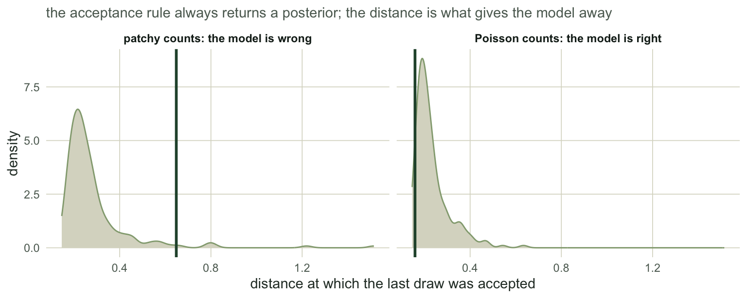
For the third question the obstacle is the acceptance rule. Keeping your best 0.25 per cent returns a full posterior whatever the data look like. The distance at which those draws came in is what gives the model away. If the model can produce data like yours, the observed summaries lie on the surface the simulator can reach, and the nearest simulations land as close to them as they land to data the model generates itself. If it cannot, the observed summaries sit off that surface, everything is far away, and the accepted distance is larger than the fitted model can explain. Compare it with a parametric bootstrap from the accepted draws: that is model criticism through the ABC discrepancy itself (Ratmann et al. 2009; Frazier, Robert and Rousseau 2020).

The misspecification is the one every ecologist has. Counts are patchy, not Poisson. The truth below is the same Ricker process with negative binomial counting, swept from mild to severe; the fitted model insists on Poisson throughout.

sim_nb <- function(log_r, sigma, size, T = 50, phi = 10, N0 = 1) {
  M <- length(log_r); N <- rep(N0, M); Y <- matrix(0L, M, T)
  for (t in seq_len(T)) {
    N <- exp(log_r) * N * exp(-N + rnorm(M, 0, sigma))
    Y[, t] <- rnbinom(M, mu = phi * N, size = size)
  }
  Y
}

set.seed(2911)
M_pool  <- 20000
Th_p    <- prior(M_pool)
Sj      <- sweep(summ(sim_ricker(Th_p[, 1], Th_p[, 2]))[, fit_cols], 2, sc[fit_cols], "/")
k_acc   <- 50                                   # the closest 0.25 per cent
dist_to <- function(s0) sqrt(rowSums(sweep(Sj, 2, s0[fit_cols] / sc[fit_cols], "-")^2))

abc_gof <- function(y0, B = 30) {
  s0   <- drop(summ(y0))
  d    <- dist_to(s0)
  acc  <- order(d)[seq_len(k_acc)]
  dobs <- d[acc[k_acc]]                         # distance the last accepted draw came in at
  th   <- Th_p[acc[sample.int(k_acc, B, replace = TRUE)], , drop = FALSE]
  Yr   <- sim_ricker(th[, 1], th[, 2])          # data the fitted model itself produces
  drep <- vapply(seq_len(B),
                 function(b) sort(dist_to(drop(summ(Yr[b, , drop = FALSE]))))[k_acc],
                 numeric(1))
  ci <- quantile(Th_p[acc, 1], c(0.05, 0.95))
  structure(c(p = mean(drep >= dobs), dobs = dobs, logr = mean(Th_p[acc, 1]),
              sd = sd(Th_p[acc, 1]), cover = as.numeric(ci[1] <= 3.8 && 3.8 <= ci[2])),
            drep = drep)
}

set.seed(29111)
sizes <- c(Inf, 10, 3, 1)
ms <- do.call(rbind, lapply(sizes, function(sz) {
  r <- replicate(40, {
    y0 <- if (is.infinite(sz)) sim_ricker(3.8, 0.3) else sim_nb(3.8, 0.3, size = sz)
    abc_gof(y0)
  })
  data.frame(size = sz, var_ratio = ifelse(is.infinite(sz), 1, 1 + 39 / sz),
             logr = mean(r["logr", ]), scatter = sd(r["logr", ]),
             post_sd = mean(r["sd", ]), cover90 = mean(r["cover", ]),
             alarm = mean(r["p", ] < 0.05), dobs = mean(r["dobs", ]))
}))
print(ms, digits = 3, row.names = FALSE)

 size var_ratio logr scatter post_sd cover90 alarm  dobs
  Inf       1.0 3.77   0.127   0.125   0.825 0.050 0.230
   10       4.9 3.75   0.171   0.125   0.675 0.175 0.290
    3      14.0 3.77   0.369   0.160   0.400 0.350 0.445
    1      40.0 3.60   0.370   0.143   0.325 0.375 0.580

Read logr first, because it is the surprise. The posterior mean of log_r is 3.77, 3.75, 3.77, 3.6 across the four arms, against a truth of 3.8. Overdispersion of 40 times the Poisson variance leaves the estimate essentially where it was. If you only ever looked at the point estimate you would never know anything had happened.

Now read scatter and post_sd together. The estimate wanders from data set to data set by 0.127 under Poisson counts and by 0.37 under severe overdispersion, a factor of 2.9, while the posterior standard deviation the analysis reports moves only from 0.125 to 0.143. The interval stops describing the estimator. Its coverage drops from 82 per cent to 32 per cent: the 90 per cent credible interval covers a little under half the time. That is the harm from misspecification here, and it is not bias. It is a confident interval around a number that jumps. It is also exactly what the theory says to expect: under a misspecified simulator the ABC posterior concentrates on a pseudo-true value and its credible sets stop having frequentist coverage (Frazier, Robert and Rousseau 2020). The table is that sentence with numbers in it.

The acceptance distance check sees it. On well specified data it fires in 5 per cent of replicates, at or below its nominal 5 per cent, and at size = 1 it fires in 38 per cent, with the accepted distance itself rising from 0.23 to 0.58. It is not a licence. Mild overdispersion, size = 10, is already 4.9 times the Poisson variance and already costs 15 points of coverage, and the check fires in 18 per cent of replicates, which is no signal at all. The check catches the wreck and misses the dent, and every check on a two dimensional surface in a four dimensional summary space will behave that way.

And the sting: the calibration check of Check 1 passes on all four rows. It simulates its own data from the Poisson model, so nothing in the sweep above can reach it. A rank histogram and a coverage curve, both flat, both correct, on an analysis whose interval covers 32 per cent of the time on the data you actually have.

Figure 3: The acceptance distance as a test statistic, both panels on one scale. Grey: distances reached on data the fitted model itself produces. Green line: the distance at which the real analysis accepted its draws.

What each check is worth

Three checks, three different objects, and no one of them substitutes for another.

The rank histogram audits the sampler. It needs no observed data, which is exactly its limit: it cannot fail because your model is wrong. Read its shape rather than its coverage number, and read the posterior width beside it, because a procedure that returns the prior passes it perfectly.

The posterior width audits the answer. It is not a test, it has no p-value, and it is the only thing in this post that would have told you that the mean count says nothing about process noise. Compare it with the prior width, parameter by parameter, and report both.

The acceptance distance audits the model. It is the only check here that can fail because the world is not your simulator, and it has the power curve you would expect: sharp when the model is badly wrong, silent when the error is mild, and mild errors are not free.

Underneath all three sits the limit that choosing summary statistics already named. Every check in this post reaches the data through the summaries. A misspecification no summary responds to is invisible to all of them, and a parameter the summaries do not identify has a posterior near its prior, which calibration will bless. That is not a defect of the diagnostics. It is the price of an analysis that sees the data through four numbers, and the diagnostics can no more escape it than the estimate can.

One repair is not available: making the tolerance small enough that the problem goes away. The sampler post priced that on this same model. The whole gain available to any sampler over plain rejection is about a factor of ten, the best sequential sampler collected under a fifth of it, and tightening the tolerance lifts the ceiling by about a third while multiplying the simulation bill by four. The tolerance you can afford is the tolerance you have to check at.

Where to go next

Run the calibration loop at the acceptance rate you can actually afford, and read the width column next to the histogram. If the histogram is flat there, you have a sampler you can trust at that price. If it is not, you have learned something concrete and the direction of the dent tells you which way the posterior leans.

If the acceptance distance test fires, the answer is not a better sampler. It is a better simulator: a negative binomial observation layer here, an extra process there. ABC makes that cheap, because a model you can simulate is a model you can fit, and the cost of the extra layer is a parameter and a summary that identifies it. The check that fired is also the check that will tell you whether the repair worked.

References

Cook, Gelman and Rubin 2006 Journal of Computational and Graphical Statistics 15(3):675-692 (10.1198/106186006X136976)

Frazier, Robert and Rousseau 2020 Journal of the Royal Statistical Society Series B 82(2):421-444 (10.1111/rssb.12356)

Prangle, Blum, Popovic and Sisson 2014 Australian and New Zealand Journal of Statistics 56(4):309-329 (10.1111/anzs.12087)

Ratmann, Andrieu, Wiuf and Richardson 2009 Proceedings of the National Academy of Sciences 106(26):10576-10581 (10.1073/pnas.0807882106)

Wood 2010 Nature 466(7310):1102-1104 (10.1038/nature09319)

Related tutorials

• Approximate Bayesian computation from scratch
• Choosing summary statistics for ABC
• ABC-MCMC and sequential ABC samplers
• Checking predictive calibration