Checking a multiple-testing analysis

Three diagnostics for a false-discovery-rate analysis: the p-value histogram, estimating the null proportion, and the sensitivity of the discovery set.

The previous three tutorials chose an error rate and a correction: Bonferroni and Holm for the family-wise error, Benjamini-Hochberg for the false discovery rate, Benjamini-Yekutieli when the tests are correlated. This closing post asks how to check the analysis before you trust it. Three diagnostics carry most of the weight: the shape of the p-value histogram, an estimate of how many nulls are true, and the sensitivity of the discovery set to the choices you made. All are base R.

Setup

The p-value histogram

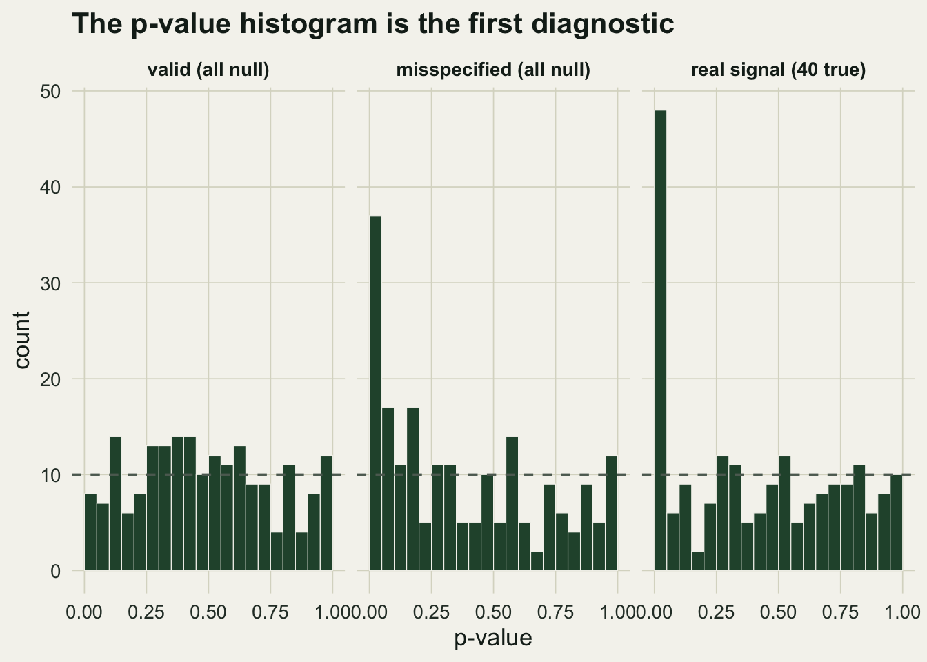
Every correction in this series takes p-values as its raw material and assumes they are valid: under a true null, a p-value is uniform on the unit interval. The single most useful check is to plot the histogram of all your p-values and look at its shape. A valid analysis with some real effects shows a flat carpet from the null tests plus a spike near zero from the true ones. A flat histogram with no spike means nothing is there. A histogram that rises toward zero when nothing should be there means the p-values are not valid, usually because unmodelled dependence or overdispersion has made the tests anticonservative.

We simulate three screens of 200 taxa: all nulls with valid tests, all nulls with overdispersed statistics analysed as if standard normal (the pseudoreplication trap), and a real mixture of 40 true effects among 160 nulls.

m <- 200; m1 <- 40; m0 <- m - m1; mu <- 3
nonnull <- c(rep(TRUE, m1), rep(FALSE, m0))
gof_unif <- function(p, B = 10){
  ct <- table(cut(p, breaks = seq(0, 1, length.out = B + 1), include.lowest = TRUE))
  chisq.test(as.numeric(ct))$p.value
}
set.seed(303)
p_null <- 2 * pnorm(-abs(rnorm(m)))                            # valid, all null
p_mis  <- 2 * pnorm(-abs(rnorm(m, sd = 1.4)))                  # overdispersed, all null
p_mix  <- 2 * pnorm(-abs(rnorm(m, mean = ifelse(nonnull, mu, 0))))  # 40 true effects
c(valid_GOF = round(gof_unif(p_null), 3),
  misspecified_GOF = signif(gof_unif(p_mis), 3),
  mixture_GOF = signif(gof_unif(p_mix), 3))

       valid_GOF misspecified_GOF      mixture_GOF 
        4.47e-01         7.99e-13         7.36e-11 

c(frac_below_05_valid = mean(p_null < 0.05),
  frac_below_05_misspecified = mean(p_mis < 0.05),
  frac_below_05_mixture = mean(p_mix < 0.05))

       frac_below_05_valid frac_below_05_misspecified 
                     0.040                      0.185 
     frac_below_05_mixture 
                     0.240 

A chi-square test of uniformity gives the valid nulls a comfortable p-value of 0.447, and rejects uniformity decisively for both the misspecified case and the real mixture. The two rejections mean opposite things, which is why the picture matters. The misspecified histogram rises toward zero even though not one taxon has a real effect: 18 per cent of its p-values fall below 0.05, against the 4 per cent you expect, close to the 0.162 predicted for statistics inflated this way. Feed those p-values to any correction and it will report discoveries that are artefacts of the unmodelled variance, not biology.

d <- data.frame(p = c(p_null, p_mis, p_mix),
  panel = factor(rep(c("valid (all null)","misspecified (all null)","real signal (40 true)"),
                     each = m),
                 levels = c("valid (all null)","misspecified (all null)","real signal (40 true)")))
ggplot(d, aes(p)) +
  geom_histogram(breaks = seq(0, 1, .05), fill = c_bh, colour = te_paper, linewidth = .2) +
  facet_wrap(~panel) +
  geom_hline(yintercept = m/20, linetype = "dashed", colour = te_faint) +
  labs(x = "p-value", y = "count", title = "The p-value histogram is the first diagnostic") +
  theme_te()

Figure 1: Histograms of p-values for a valid all-null screen, an overdispersed all-null screen, and a screen with forty real effects. Uniform under the null; a spike with no signal (centre) flags misspecification.

Estimating the proportion of true nulls

Benjamini-Hochberg implicitly assumes every null could be true, which is conservative when many are not. Storey’s approach estimates the true-null proportion pi0 directly: high p-values are almost all from nulls, so pi0_hat(lambda) = #{p > lambda} / (m (1 - lambda)) for some cut lambda. Adaptive procedures then run BH at the sharper level q / pi0_hat.

pi0_hat <- function(p, lam) min(1, mean(p > lam) / (1 - lam))
sweep <- sapply(c(0.3, 0.5, 0.8), function(l)
  c(mixture = pi0_hat(p_mix, l), valid_null = pi0_hat(p_null, l),
    misspecified = pi0_hat(p_mis, l)))
colnames(sweep) <- c("lambda=0.3","lambda=0.5","lambda=0.8")
round(sweep, 3)

             lambda=0.3 lambda=0.5 lambda=0.8
mixture           0.829       0.85      0.875
valid_null        1.000       0.93      0.875
misspecified      0.729       0.71      0.750

On the real mixture the estimate lands near the truth of 0.8 (between 0.829 and 0.875 across the cut), and adaptive BH would gain a little power. But the estimate depends on lambda, which is a choice, and it inherits the same fragility as the histogram. On the misspecified screen pi0_hat drops to around 0.71, falsely implying that a quarter of the taxa have real effects when none do. The estimator trusts that the nulls are uniform; when they are not, it is misled in exactly the way the histogram exposes. The diagnostic that catches the problem is the picture, not the point estimate.

The discovery set is a function of your choices

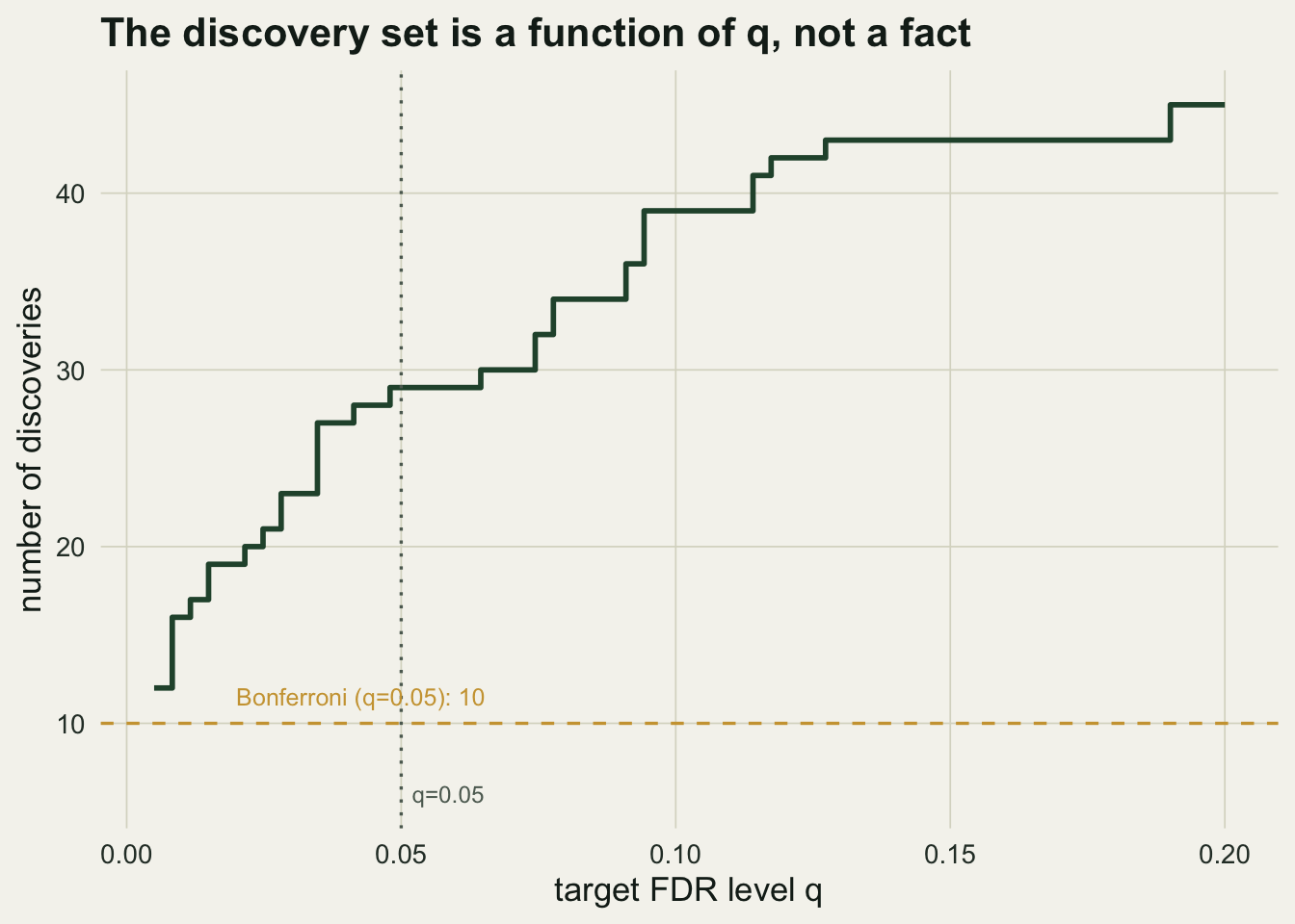
The deepest check is to see how much the result depends on the decisions you could have made differently. The number of discoveries is a function of the target level q, and of the far larger choice between controlling the family-wise error and the false discovery rate.

set.seed(2718)
z <- rnorm(m, mean = ifelse(nonnull, mu, 0)); p <- 2 * pnorm(-abs(z))
padj <- p.adjust(p, "BH")
q_grid <- c(0.01, 0.02, 0.05, 0.10, 0.15, 0.20)
Rq <- sapply(q_grid, function(qq) sum(padj <= qq))
setNames(Rq, q_grid)

0.01 0.02 0.05  0.1 0.15  0.2 
  16   20   29   39   43   45 

c(bonferroni_at_05 = sum(p.adjust(p, "bonferroni") < 0.05), bh_at_05 = sum(padj <= 0.05))

bonferroni_at_05         bh_at_05 
              10               29 

Sweeping q from 0.01 to 0.20 moves the discovery count from 16 to 45. On the very same data, controlling the family-wise error with Bonferroni yields 10 discoveries where the false discovery rate yields 29: the choice of error rate moves the answer far more than any wiggle in q. And no procedure among them identifies which taxa are the real effects. Of the 40 genuine effects here, 27 are recovered at q = 0.05; the rest sit below the line, indistinguishable from nulls at this threshold.

The same logic localises a single finding. A taxon enters the discovery set at the q equal to its own adjusted p-value, its tipping point.

ord <- order(padj)
borderline <- ord[which(padj[ord] > 0.05)[1]]
round(padj[borderline], 4)

[1] 0.0632

The borderline taxon here has an adjusted p-value of 0.0632, so it is a discovery at q = 0.07 but not at q = 0.05. Whether you report it is a decision about how many false leads you will tolerate, not a fact the data settle.

qg <- seq(0.005, 0.20, length.out = 60)
Rqc <- sapply(qg, function(qq) sum(padj <= qq))
ggplot(data.frame(q = qg, R = Rqc), aes(q, R)) +
  geom_step(colour = c_bh, linewidth = 1) +
  geom_hline(yintercept = sum(p.adjust(p, "bonferroni") < 0.05),
             linetype = "dashed", colour = c_bonf) +
  geom_vline(xintercept = 0.05, linetype = "dotted", colour = te_faint) +
  annotate("text", x = 0.02, y = sum(p.adjust(p, "bonferroni") < 0.05) + 1.5,
           label = "Bonferroni (q=0.05): 10", colour = c_bonf, hjust = 0, size = 3.3) +
  annotate("text", x = 0.052, y = 6, label = "q=0.05", colour = te_faint, hjust = 0, size = 3.2) +
  labs(x = "target FDR level q", y = "number of discoveries",
       title = "The discovery set is a function of q, not a fact") +
  theme_te()

Figure 2: Number of Benjamini-Hochberg discoveries as a function of the target level q, with the Bonferroni count for comparison. The discovery set is a monotone function of a choice, not a fixed list.

What the checks do and do not settle

The three diagnostics constrain the analysis without proving it correct. The histogram tells you whether the p-values are valid, and it is the check that survives when the null distribution is wrong; the null-proportion estimate sharpens power but trusts the same uniformity and is misled when it fails; the sensitivity sweep shows that the discovery set is a decision at a chosen threshold under a chosen error rate, not a list of true effects. A multiple-testing correction never hands you the taxa that matter. It hands you a ranked, thresholded set whose contents move with q, with the error rate you picked, and with the dependence you were willing to assume. Reporting those choices alongside the discoveries is what makes the result honest.

References

Storey JD 2002. J R Stat Soc Ser B 64(3):479-498 (10.1111/1467-9868.00346).

Storey JD, Tibshirani R 2003. Proc Natl Acad Sci USA 100(16):9440-9445 (10.1073/pnas.1530509100).

Benjamini Y, Hochberg Y 1995. J R Stat Soc Ser B 57(1):289-300 (10.1111/j.2517-6161.1995.tb02031.x).

Murtaugh PA 2014. Ecology 95(3):611-617 (10.1890/13-0590.1).

Gotelli NJ, Ellison AM 2013. A Primer of Ecological Statistics, 2nd ed. Sinauer Associates. ISBN 978-1-60535-064-6.

Related tutorials

• The false discovery rate and Benjamini-Hochberg
• Family-wise error and the Bonferroni correction
• Dependence and the Benjamini-Yekutieli correction
• GLM residual diagnostics