---
title: "Family-wise error and the Bonferroni correction"
description: "Why running many ecological tests at 0.05 inflates the false-positive rate, and how the Bonferroni, Holm and Sidak corrections rein it back in, in base R."
date: "2026-05-29 11:00"
categories: [R, multiple testing, hypothesis testing, ecology tutorial]
image: thumbnail.png
image-alt: "Family-wise error rate climbing towards one as the number of tests grows, leaving the flat dashed five per cent per-test level far behind."
date-modified: "2026-09-27"
---
*Corrected 27 September 2026: the power figure's title said correction costs "a little" power, but the bars it shows record a large drop in power; the title now says only that correction trades power for controlled error.*
Run one test at the five per cent level and you accept a one-in-twenty chance of a false positive. Run twenty tests and that chance is no longer one in twenty. Ecologists reach the many-test situation constantly: a difference tested across every taxon in a table, every pairwise comparison between sites, every candidate driver in a screen. This post shows how fast the error compounds, and works through the corrections that hold it in check, all in base R.
```{r}
#| label: setup
#| code-fold: true
#| code-summary: "Setup: packages, colours and plot theme"
#| results: hide
#| message: false
#| warning: false
library(ggplot2)
te_ink<-"#16241d"; te_body<-"#2c3a31"; te_forest<-"#275139"; te_faint<-"#5d6b61"
te_paper<-"#f5f4ee"; te_line<-"#dad9ca"
c_raw<-"#b5534e"; c_bonf<-"#cda23f"; c_holm<-"#2f8f63"
theme_te <- function(base=13) theme_minimal(base_size=base) +
  theme(plot.background=element_rect(fill=te_paper,colour=NA),
        panel.background=element_rect(fill=te_paper,colour=NA),
        panel.grid.minor=element_blank(),
        panel.grid.major=element_line(colour=te_line,linewidth=.3),
        axis.text=element_text(colour=te_body), axis.title=element_text(colour=te_ink),
        plot.title=element_text(colour=te_ink,face="bold"),
        plot.subtitle=element_text(colour=te_faint),
        legend.text=element_text(colour=te_body), legend.title=element_text(colour=te_ink),
        strip.text=element_text(colour=te_ink,face="bold"))
```
## How fast the error grows
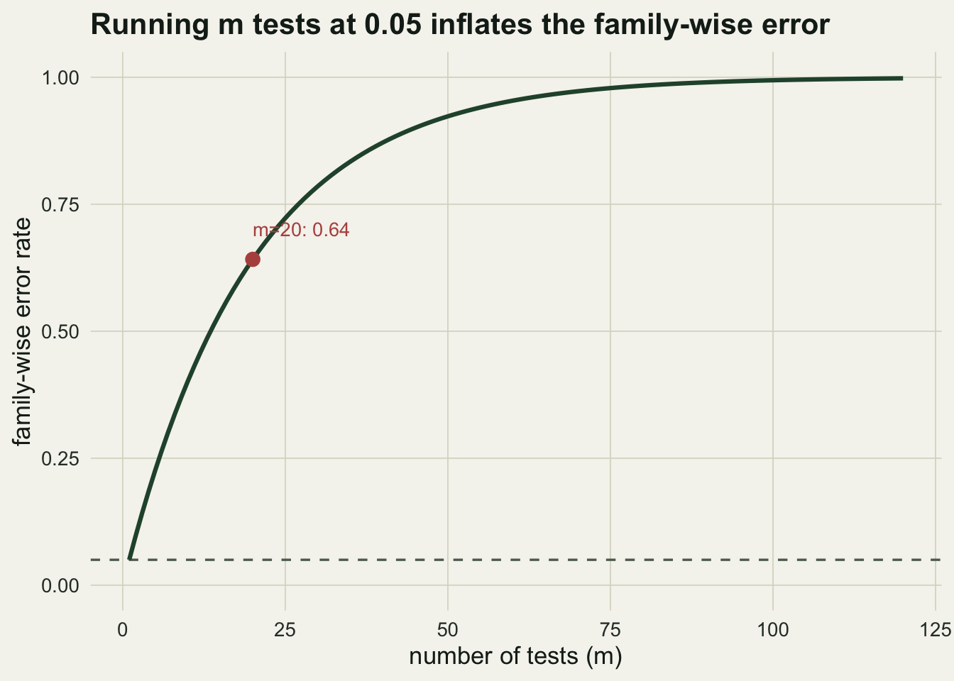
If you run `m` independent tests and every null is true, the probability that at least one comes back significant at level `alpha` is one minus the probability that none does:
$$\text{FWER} = 1 - (1-\alpha)^m.$$
This is the family-wise error rate: the chance of one or more false positives across the whole family of tests.
```{r}
#| label: fwer-grid
alpha <- 0.05
m_grid <- c(1, 5, 10, 20, 50, 100)
fwer <- 1 - (1 - alpha)^m_grid
setNames(round(fwer, 3), m_grid)
```
At `m = 20` the family-wise error is already `r round(1-(1-alpha)^20, 3)`, and by `m = 100` it is `r round(1-(1-alpha)^100, 3)`. A screen across a hundred taxa is almost guaranteed to hand you a "significant" result even when nothing is going on.
```{r}
#| label: fig-fwer
#| fig-cap: "Family-wise error rate as a function of the number of tests, when every null is true. The nominal five per cent level (dashed) is the per-test rate, not the family rate."
#| fig-alt: "A rising curve of family-wise error against number of tests, crossing 0.64 at m equals 20 and approaching one by m equals 100, with a flat dashed line at 0.05."
mg <- seq(1, 120)
ggplot(data.frame(m=mg, fwer=1-(1-alpha)^mg), aes(m, fwer)) +
  geom_hline(yintercept=alpha, linetype="dashed", colour=te_faint) +
  geom_line(colour=te_forest, linewidth=1.1) +
  geom_point(data=data.frame(m=20, fwer=1-(1-alpha)^20), size=3, colour=c_raw) +
  annotate("text", x=22, y=1-(1-alpha)^20-.04, label="m=20: 0.64",
           colour=c_raw, hjust=0, size=3.6) +
  scale_y_continuous(limits=c(0,1)) +
  labs(x="number of tests (m)", y="family-wise error rate",
       title="Running m tests at 0.05 inflates the family-wise error") +
  theme_te()
```
## One run, twenty null taxa
To see the trap in action, simulate twenty taxa measured in two habitats with `r 30` replicates each, drawn from the same distribution so that every null is genuinely true. We test each taxon with a two-sample t-test.
```{r}
#| label: single-run
set.seed(1)
mtax <- 20; n <- 30
grpA <- matrix(rnorm(mtax*n), n, mtax)   # habitat A
grpB <- matrix(rnorm(mtax*n), n, mtax)   # habitat B, identical distribution
pvals <- sapply(1:mtax, function(j) t.test(grpA[,j], grpB[,j])$p.value)
raw_hits <- which(pvals < alpha)
raw_hits
round(sort(pvals)[1:3], 4)
```
Nothing differs, yet the raw analysis flags `r length(raw_hits)` taxa (numbers `r paste(raw_hits, collapse=" and ")`), with the smallest p-value at `r round(min(pvals),4)`. These are pure false positives. Reporting them as findings is the multiple-comparisons mistake.
## Bonferroni, Holm and Sidak
The Bonferroni correction tests each hypothesis at `alpha / m` instead of `alpha`. It bounds the family-wise error at `alpha` under any dependence structure, at the price of a very small per-test threshold. Holm's step-down procedure is a sharper version: sort the p-values, and compare the k-th smallest against `alpha / (m - k + 1)`. It controls the same family-wise error but rejects at least as much as Bonferroni, so there is no reason to prefer plain Bonferroni over it. Sidak's threshold, `1 - (1 - alpha)^(1/m)`, is exact under independence.
Each is a few lines by hand, and each matches R's built-in `p.adjust`.
```{r}
#| label: corrections
bonf <- function(p) pmin(p * length(p), 1)
holm <- function(p){
  m <- length(p); o <- order(p)
  adj <- cummax((m - seq_len(m) + 1) * p[o])
  out <- numeric(m); out[o] <- pmin(adj, 1); out
}
sidak_thr <- 1 - (1 - alpha)^(1/mtax)
c(bonferroni = max(abs(bonf(pvals) - p.adjust(pvals, "bonferroni"))),
  holm       = max(abs(holm(pvals) - p.adjust(pvals, "holm"))))
```
Applied to the run above, Bonferroni uses a threshold of `alpha / m` = `r alpha/mtax`, and the Sidak threshold is `r round(sidak_thr, 5)`. Both leave `r sum(p.adjust(pvals,"bonferroni")<alpha)` taxa significant, and so does Holm: the two spurious hits are gone.
## Do the corrections actually control the error?
A short Monte Carlo makes the guarantee concrete. Generate the complete-null scenario three thousand times and record, for each method, whether at least one of the twenty tests is rejected.
```{r}
#| label: mc-fwer
welch_p <- function(a, b){
  n1<-nrow(a); n2<-nrow(b); m1<-colMeans(a); m2<-colMeans(b)
  v1<-apply(a,2,var); v2<-apply(b,2,var); se2<-v1/n1+v2/n2
  tt<-(m1-m2)/sqrt(se2)
  df<-se2^2/((v1/n1)^2/(n1-1)+(v2/n2)^2/(n2-1))
  2*pt(-abs(tt), df)
}
sidak_p <- function(p) pmin(1 - (1-p)^length(p), 1)
set.seed(4242)
R <- 3000
fw <- c(raw=0, bonferroni=0, holm=0, sidak=0)
for(r in 1:R){
  A<-matrix(rnorm(mtax*n),n,mtax); B<-matrix(rnorm(mtax*n),n,mtax)
  p<-welch_p(A,B)
  fw["raw"]        <- fw["raw"]        + (min(p) < alpha)
  fw["bonferroni"] <- fw["bonferroni"] + (min(p.adjust(p,"bonferroni")) < alpha)
  fw["holm"]       <- fw["holm"]       + (min(p.adjust(p,"holm")) < alpha)
  fw["sidak"]      <- fw["sidak"]      + (min(sidak_p(p)) < alpha)
}
round(fw / R, 3)
```
The uncorrected analysis fires on `r round(fw["raw"]/R*100)` per cent of runs, tracking the `r round(1-(1-alpha)^20, 3)` predicted by the formula. Bonferroni, Holm and Sidak all sit near the nominal five per cent.
## The cost: power
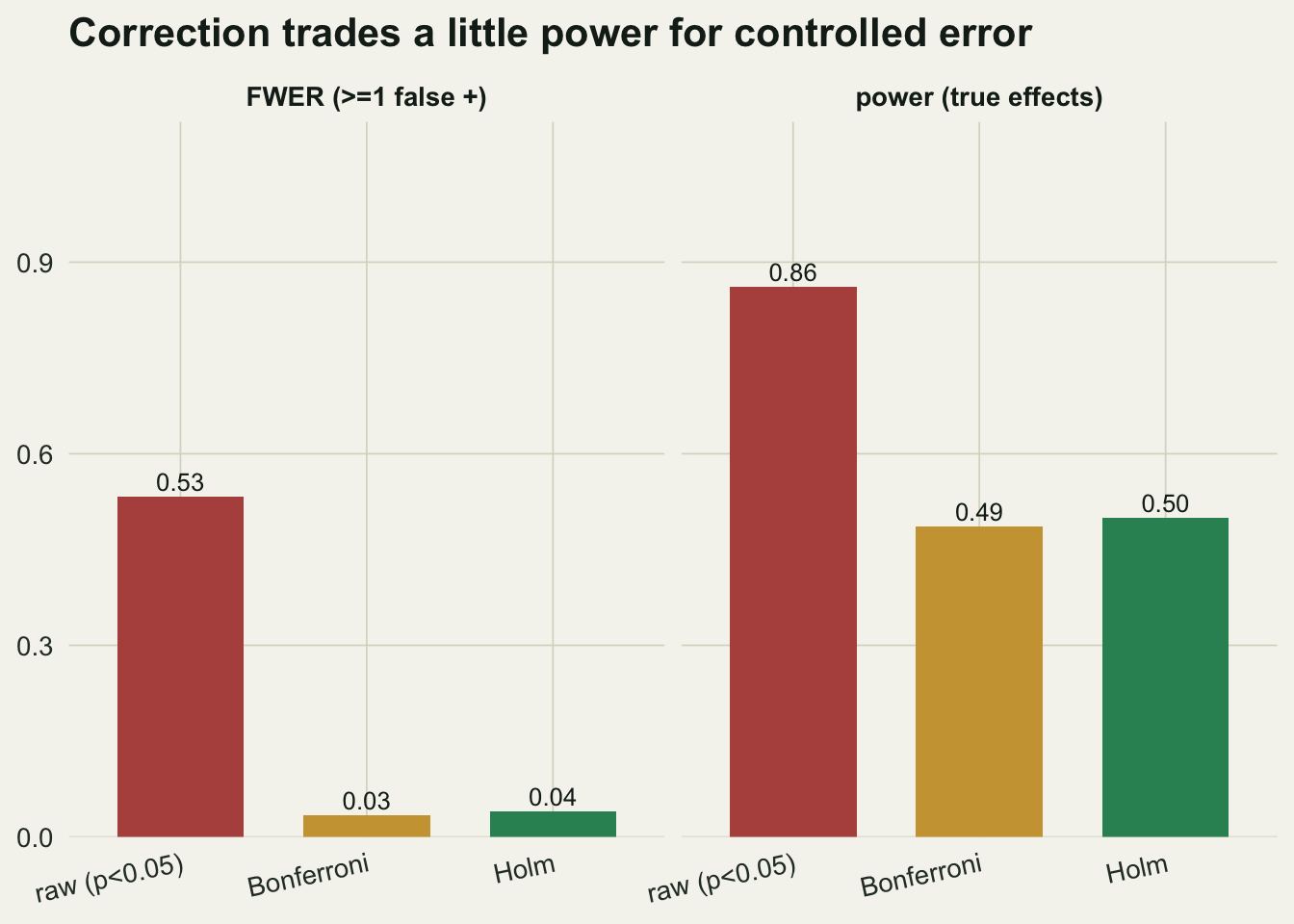
Control is not free. Shrinking the per-test threshold makes real effects harder to detect. Here five of the twenty taxa truly differ (a moderate effect of `r 0.8` standard deviations), and we track both the power to detect them and the family-wise error among the fifteen nulls.
```{r}
#| label: power-demo
set.seed(31337)
m1 <- 5; delta <- 0.8
true_eff <- c(rep(TRUE, m1), rep(FALSE, mtax - m1))
mu_vec <- rep(c(delta, 0), c(m1, mtax - m1))
Rp <- 3000
pw <- matrix(0, Rp, 3); fwv <- matrix(0, Rp, 3)
holm_never_worse <- TRUE
for(r in 1:Rp){
  A <- matrix(rnorm(mtax*n), n, mtax)
  B <- sweep(matrix(rnorm(mtax*n), n, mtax), 2, mu_vec, "+")
  p <- welch_p(A, B)
  rj <- cbind(p < alpha, p.adjust(p,"bonferroni") < alpha, p.adjust(p,"holm") < alpha)
  if(sum(rj[,3]) < sum(rj[,2])) holm_never_worse <- FALSE
  pw[r,]  <- colMeans(rj[true_eff, , drop=FALSE])
  fwv[r,] <- apply(rj[!true_eff, , drop=FALSE], 2, any)
}
power <- setNames(round(colMeans(pw), 3), c("raw","bonferroni","holm"))
fwerp <- setNames(round(colMeans(fwv), 3), c("raw","bonferroni","holm"))
rbind(power = power, fwer = fwerp)
```
```{r}
#| label: fig-power
#| fig-cap: "Power to detect five true effects and the family-wise error among the fifteen nulls, for the raw analysis and two corrections. Holm buys back a little power over Bonferroni at the same error."
#| fig-alt: "Two bar panels. Power panel: raw 0.86, Bonferroni 0.49, Holm 0.50. Family-wise error panel: raw 0.53, Bonferroni 0.03, Holm 0.04."
d <- data.frame(
  method = factor(rep(c("raw (p<0.05)","Bonferroni","Holm"), 2),
                  levels=c("raw (p<0.05)","Bonferroni","Holm")),
  metric = rep(c("power (true effects)","FWER (>=1 false +)"), each=3),
  value  = c(power, fwerp))
ggplot(d, aes(method, value, fill=method)) +
  geom_col(width=.68) + facet_wrap(~metric) +
  geom_text(aes(label=sprintf("%.2f", value)), vjust=-0.35, size=3.4, colour=te_ink) +
  scale_fill_manual(values=c(c_raw,c_bonf,c_holm), guide="none") +
  scale_y_continuous(limits=c(0,1), expand=expansion(mult=c(0,.12))) +
  labs(x=NULL, y=NULL, title="Correction trades power for controlled error") +
  theme_te() + theme(axis.text.x=element_text(angle=12, hjust=1))
```
The raw analysis has the highest power (`r power["raw"]`) but a family-wise error of `r fwerp["raw"]`: in most runs it also flags at least one of the fifteen nulls. Bonferroni cuts power to `r power["bonferroni"]` while pinning the error near five per cent. Holm recovers a little of that power (`r power["holm"]`) at the same error, and in this simulation it rejected at least as many hypotheses as Bonferroni in every single run, as the theory promises.
## The honest limit
The family-wise error rate is a strict target: it guards against even one false positive anywhere in the family. That is the right stance when a single wrong call is costly, but it is often too strict for exploratory ecology, where you scan hundreds of taxa and can tolerate a few false leads if it means finding the real ones. Holm sharpens Bonferroni without changing what it controls; neither tells you which of your significant results are the true ones. The deeper choice is which error rate to control at all. When the family is large and the goal is discovery, the false discovery rate is usually the better currency, and that is the subject of the next tutorial.
## References
Benjamini Y, Hochberg Y 1995. J R Stat Soc Ser B 57(1):289-300 (10.1111/j.2517-6161.1995.tb02031.x).
Holm S 1979. Scand J Stat 6(2):65-70 (no DOI).
Sidak Z 1967. J Am Stat Assoc 62(318):626-633 (10.1080/01621459.1967.10482935).
Aickin M, Gensler H 1996. Am J Public Health 86(5):726-728 (10.2105/AJPH.86.5.726).
Rice WR 1989. Evolution 43(1):223-225 (10.1111/j.1558-5646.1989.tb04220.x).
Moran MD 2003. Oikos 100(2):403-405 (10.1034/j.1600-0706.2003.12010.x).
Nakagawa S 2004. Behav Ecol 15(6):1044-1045 (10.1093/beheco/arh107).
Quinn GP, Keough MJ 2002. Experimental Design and Data Analysis for Biologists. Cambridge University Press. ISBN 978-0-521-00976-8.
## Related tutorials
- [Controlling the false discovery rate with Benjamini-Hochberg](../false-discovery-rate-benjamini-hochberg/)
- [Power analysis by simulation](../power-analysis-by-simulation/)
- [Linear models: t-test and ANOVA as one framework](../linear-models-t-test-anova/)
- [Pairwise PERMANOVA and post-hoc comparisons](../pairwise-permanova/)