---
title: "The false discovery rate and Benjamini-Hochberg"
description: "When you screen hundreds of taxa, Bonferroni discards real signal. Benjamini-Hochberg controls the false discovery rate instead, step by step in base R."
date: "2026-05-29 12:00"
categories: [R, multiple testing, false discovery rate, ecology tutorial]
image: thumbnail.png
image-alt: "Sorted p-values rising with rank, with a flat Bonferroni threshold near zero and a sloped Benjamini-Hochberg line admitting many more of them."
---
The [Bonferroni and Holm corrections](../family-wise-error-and-bonferroni/) guard against even a single false positive. That is the right goal for a handful of tests, but modern ecological data routinely brings hundreds: a differential-abundance screen across every taxon in a table, a genome-wide scan, a grid of environmental associations. At that scale the family-wise machinery becomes so strict that it throws away almost every real effect. This post works through the false discovery rate, a target built for large screens, and the Benjamini-Hochberg procedure that controls it, in base R.
```{r}
#| label: setup
#| code-fold: true
#| code-summary: "Setup: packages, colours and plot theme"
#| results: hide
#| message: false
#| warning: false
library(ggplot2)
te_ink<-"#16241d"; te_body<-"#2c3a31"; te_forest<-"#275139"; te_faint<-"#5d6b61"
te_paper<-"#f5f4ee"; te_line<-"#dad9ca"
c_bonf<-"#cda23f"; c_bh<-"#275139"
theme_te <- function(base=13) theme_minimal(base_size=base) +
  theme(plot.background=element_rect(fill=te_paper,colour=NA),
        panel.background=element_rect(fill=te_paper,colour=NA),
        panel.grid.minor=element_blank(),
        panel.grid.major=element_line(colour=te_line,linewidth=.3),
        axis.text=element_text(colour=te_body), axis.title=element_text(colour=te_ink),
        plot.title=element_text(colour=te_ink,face="bold"),
        plot.subtitle=element_text(colour=te_faint),
        strip.text=element_text(colour=te_ink,face="bold"))
```
## Why Bonferroni fails at scale
Suppose you test `m = 200` taxa for a difference between two conditions. The Bonferroni threshold is `alpha / m`, which for the five per cent level is `r sprintf("%.5f", 0.05/200)`. A real effect has to clear that bar to be detected, and most genuine ecological effects simply are not that strong. The correction protects you from false positives so aggressively that it also erases the true positives you set out to find.
The false discovery rate reframes the goal. Instead of controlling the chance of *any* false positive, it controls the expected *proportion* of false positives among the tests you call significant. Write the false discovery proportion as
$$\text{FDP} = \frac{\text{false rejections}}{\max(\text{total rejections},\,1)},$$
and the false discovery rate is its expectation, FDR = E[FDP]. Controlling the FDR at `q = 0.05` means that, on average, no more than five per cent of your reported discoveries are false. You accept a few wrong calls in exchange for finding far more of the real effects.
## The Benjamini-Hochberg procedure
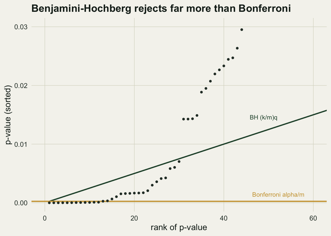
Benjamini and Hochberg (1995) give a step-up rule. Sort the p-values from smallest to largest, and find the largest rank `k` for which the k-th smallest p-value still sits below the sloped line `(k / m) * q`. Reject every hypothesis up to that rank. It is a few lines by hand, and matches `p.adjust(..., "BH")`.
```{r}
#| label: bh-fun
BH <- function(p, q = 0.05){
  m <- length(p); o <- order(p); s <- p[o]
  below <- s <= (seq_len(m) / m) * q
  k <- if(any(below)) max(which(below)) else 0
  rej <- rep(FALSE, m); if(k > 0) rej[o[seq_len(k)]] <- TRUE
  rej
}
set.seed(99); p_chk <- runif(50)^2
identical(BH(p_chk, 0.1), p.adjust(p_chk, "BH") <= 0.1)
```
## One screen of two hundred taxa
We model each taxon by a test statistic: under the null it is standard normal, and for a taxon with a real effect it is shifted. Here `r 40` of the `r 200` taxa truly differ.
```{r}
#| label: single-run
m <- 200; m1 <- 40; m0 <- m - m1; mu <- 3; q <- 0.05
nonnull <- c(rep(TRUE, m1), rep(FALSE, m0))
set.seed(77)
z <- rnorm(m, mean = ifelse(nonnull, mu, 0))
p <- 2 * pnorm(-abs(z))                     # two-sided p-values
bonf_rej <- p.adjust(p, "bonferroni") < q
bh_rej   <- BH(p, q)
bh_thr   <- { s <- sort(p); below <- s <= (seq_len(m)/m)*q
              if(any(below)) s[max(which(below))] else 0 }
fdp <- function(rej) if(sum(rej) == 0) 0 else sum(rej & !nonnull) / sum(rej)
c(bonferroni_rejections = sum(bonf_rej), bonferroni_true = sum(bonf_rej & nonnull),
  bh_rejections = sum(bh_rej), bh_true = sum(bh_rej & nonnull), bh_fdp = round(fdp(bh_rej), 3))
```
Bonferroni finds `r sum(bonf_rej)` of the `r m1` real effects and makes no false calls. Benjamini-Hochberg finds `r sum(bh_rej & nonnull)` of them, with `r sum(bh_rej & !nonnull)` of its rejections false: a false discovery proportion of `r round(fdp(bh_rej),3)` against the threshold `q`. BH controls that proportion on average across repeated screens, not in any single run, so one run can land on either side of `q`. The reason is the threshold. Bonferroni fixes it at `r sprintf("%.5f", q/m)`, while BH lets it rise to the sloped line: here the effective cutoff is a p-value of `r round(bh_thr, 5)`, roughly `r round(bh_thr/(q/m))` times larger.
```{r}
#| label: fig-bh
#| fig-cap: "The sorted p-values against their rank, with the flat Bonferroni threshold and the sloped Benjamini-Hochberg line. BH rejects every hypothesis up to the highest rank at which a p-value still falls below the sloped line."
#| fig-alt: "A scatter of sorted p-values rising with rank. A flat gold line sits near zero (Bonferroni) and a steeper green line (BH) admits far more of the low-rank points."
so <- sort(p); rank <- seq_len(m)
ggplot(data.frame(rank = rank, p = so), aes(rank, p)) +
  geom_line(data = data.frame(rank = rank, y = (rank/m)*q), aes(rank, y),
            colour = c_bh, linewidth = .9) +
  geom_hline(yintercept = q/m, colour = c_bonf, linewidth = .9) +
  geom_point(size = 1.1, colour = te_body) +
  coord_cartesian(xlim = c(0, 60), ylim = c(0, 0.03)) +
  annotate("text", x = 58, y = q/m + .0012, label = "Bonferroni alpha/m",
           colour = c_bonf, hjust = 1, size = 3.3) +
  annotate("text", x = 52, y = (52/m)*q + .0016, label = "BH (k/m)q",
           colour = c_bh, hjust = 1, size = 3.3) +
  labs(x = "rank of p-value", y = "p-value (sorted)",
       title = "Benjamini-Hochberg rejects far more than Bonferroni") +
  theme_te()
```
## Does it actually control the rate?
A single run tells you little about an expectation. Repeat the screen three thousand times and average the false discovery proportion and the power.
```{r}
#| label: mc
set.seed(2024)
R <- 3000
fdp_bh <- fdp_bf <- pow_bh <- pow_bf <- numeric(R)
for(r in 1:R){
  z <- rnorm(m, mean = ifelse(nonnull, mu, 0)); p <- 2 * pnorm(-abs(z))
  rb <- BH(p, q); rf <- p.adjust(p, "bonferroni") < q
  fdp_bh[r] <- if(sum(rb) == 0) 0 else sum(rb & !nonnull) / sum(rb)
  fdp_bf[r] <- if(sum(rf) == 0) 0 else sum(rf & !nonnull) / sum(rf)
  pow_bh[r] <- mean(rb[nonnull]); pow_bf[r] <- mean(rf[nonnull])
}
fdr_bh <- mean(fdp_bh); fdr_bf <- mean(fdp_bf)
power_bh <- mean(pow_bh); power_bf <- mean(pow_bf)
round(c(bh_FDR = fdr_bh, bh_power = power_bh, bonf_FDR = fdr_bf, bonf_power = power_bf), 4)
```
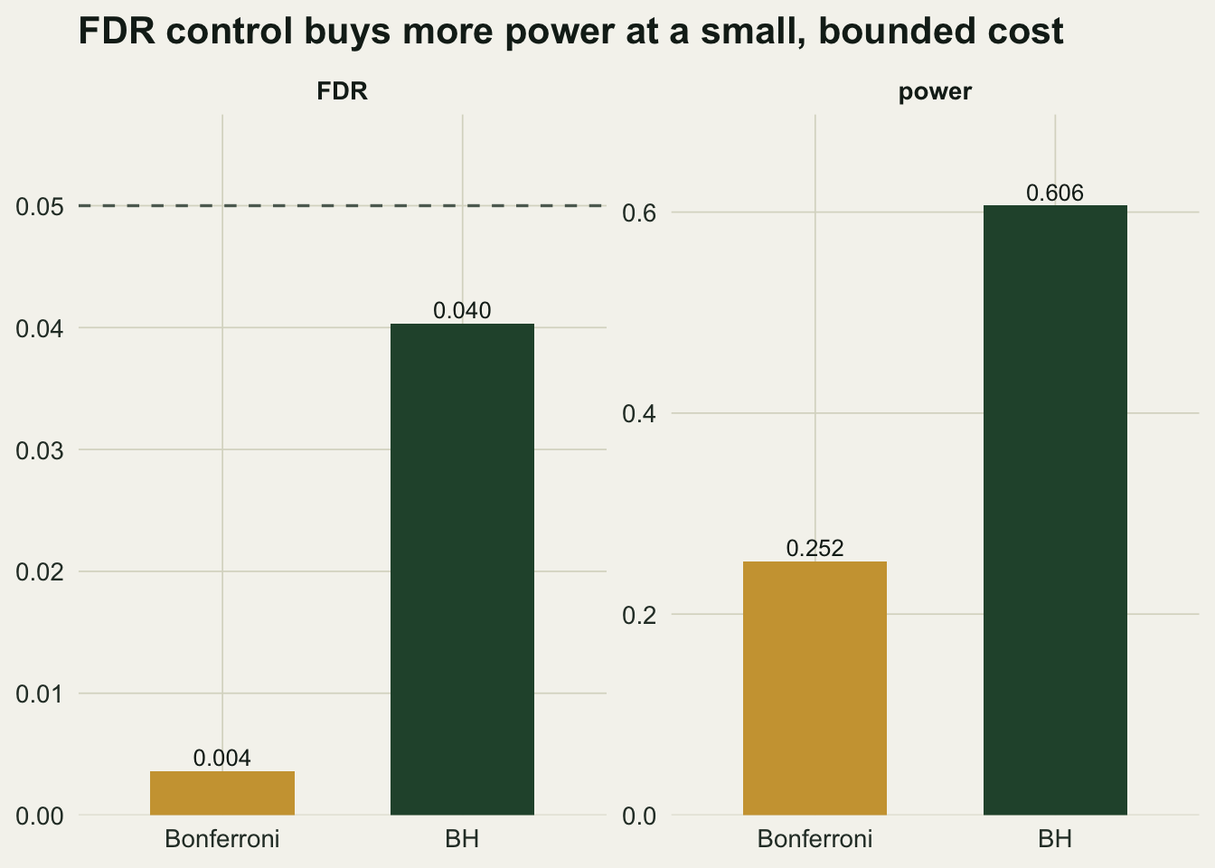
Benjamini-Hochberg holds the false discovery rate at `r round(fdr_bh,4)`, essentially at its theoretical value of `r round(q*m0/m,4)` (the guarantee is FDR at most `(m0/m) * q`, slightly below `q` because some tests are genuinely non-null). Its power is `r round(power_bh,3)`, about `r round(power_bh/power_bf,1)` times the Bonferroni power of `r round(power_bf,3)`.
```{r}
#| label: fig-fdr-power
#| fig-cap: "False discovery rate and power for Bonferroni and Benjamini-Hochberg over three thousand screens. BH keeps the rate below q (dashed) while detecting far more true effects."
#| fig-alt: "Two bar panels. Power: Bonferroni 0.25, BH 0.61. FDR: Bonferroni near zero, BH at 0.04, both under the dashed 0.05 line."
d <- data.frame(
  method = factor(rep(c("Bonferroni","BH"), 2), levels = c("Bonferroni","BH")),
  metric = rep(c("power","FDR"), each = 2),
  value  = c(power_bf, power_bh, fdr_bf, fdr_bh))
ggplot(d, aes(method, value, fill = method)) +
  geom_col(width = .6) + facet_wrap(~metric, scales = "free_y") +
  geom_text(aes(label = sprintf("%.3f", value)), vjust = -0.35, size = 3.4, colour = te_ink) +
  geom_hline(data = data.frame(metric = "FDR", yint = q), aes(yintercept = yint),
             linetype = "dashed", colour = te_faint) +
  scale_fill_manual(values = c(c_bonf, c_bh), guide = "none") +
  scale_y_continuous(expand = expansion(mult = c(0, .15))) +
  labs(x = NULL, y = NULL, title = "FDR control buys more power at a small, bounded cost") +
  theme_te()
```
## The honest limit
The false discovery rate is not the family-wise error rate, and switching to it is a genuine change of goal, not a free lunch. You are now accepting that some fraction of your reported discoveries are wrong; `q` sets that fraction, and it is a choice you make, not a property of the data. The rate is also an *average*. Across the three thousand screens above the realised false discovery proportion had a standard deviation of `r round(sd(fdp_bh),3)`, so any single study can land well above or below `q` even when the procedure is working exactly as designed. And like every correction here, BH ranks and thresholds your p-values; it never tells you which specific taxa are the true effects. Its FDR guarantee also assumes the tests are independent or positively dependent, an assumption that fails quietly when taxa co-vary. The [next tutorial](../dependence-and-fdr-benjamini-yekutieli/) takes up exactly that case.
## References
Benjamini Y, Hochberg Y 1995. J R Stat Soc Ser B 57(1):289-300 (10.1111/j.2517-6161.1995.tb02031.x).
Verhoeven KJF, Simonsen KL, McIntyre LM 2005. Oikos 108(3):643-647 (10.1111/j.0030-1299.2005.13727.x).
Storey JD, Tibshirani R 2003. Proc Natl Acad Sci USA 100(16):9440-9445 (10.1073/pnas.1530509100).
Nakagawa S 2004. Behav Ecol 15(6):1044-1045 (10.1093/beheco/arh107).
Quinn GP, Keough MJ 2002. Experimental Design and Data Analysis for Biologists. Cambridge University Press. ISBN 978-0-521-00976-8.
## Related tutorials
- [Family-wise error and the Bonferroni correction](../family-wise-error-and-bonferroni/)
- [Dependence and the Benjamini-Yekutieli correction](../dependence-and-fdr-benjamini-yekutieli/)
- [Wavelet significance and the red noise null](../wavelet-significance-and-red-noise/)
- [Checking a model-based multivariate model](../checking-a-model-based-multivariate-model/)