---
title: "Dependence and the Benjamini-Yekutieli correction"
description: "Benjamini-Hochberg assumes tests are independent or positively dependent. When ecological tests co-vary, Benjamini-Yekutieli is the safe choice, in base R."
date: "2026-05-29 13:00"
categories: [R, multiple testing, false discovery rate, ecology tutorial]
date-modified: "2026-09-27"
image: thumbnail.png
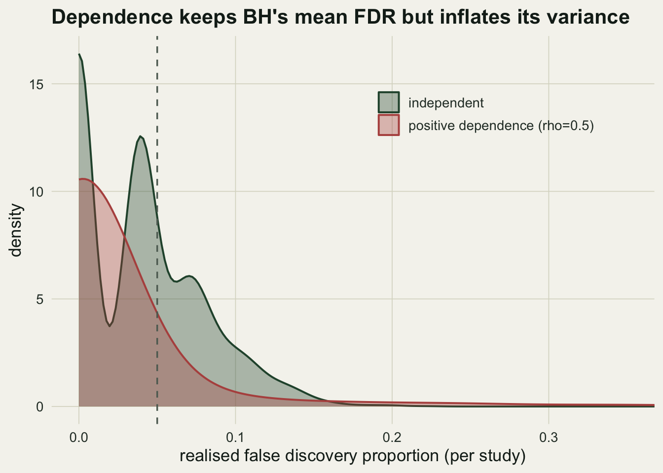
image-alt: "Two overlaid densities of the realised false discovery proportion per study, both peaking at zero: the independent one is spiky, rising again near 0.05, while the positive dependence one falls away smoothly from its peak. A dashed vertical marks 0.05."
---
*Corrected 27 September 2026: the caption of the first figure said the dependent distribution had a much wider spread, but inside the plotted window it looks narrower. The caption now says that its larger standard deviation sits in a low right tail that runs past the edge of the plot.*
The [Benjamini-Hochberg procedure](../false-discovery-rate-benjamini-hochberg/) controls the false discovery rate, but its proof needs an assumption: the tests must be independent, or positively dependent in a specific sense. Ecological tests rarely are. Taxa co-vary because they share habitat and respond to the same gradients; sites are spatially autocorrelated; abundances are linked through a fixed total. This post asks what happens to BH when the tests are correlated, and introduces the Benjamini-Yekutieli correction, which holds under any dependence at all, in base R.
```{r}
#| label: setup
#| code-fold: true
#| code-summary: "Setup: packages, colours and plot theme"
#| results: hide
#| message: false
#| warning: false
library(ggplot2)
te_ink<-"#16241d"; te_body<-"#2c3a31"; te_forest<-"#275139"; te_faint<-"#5d6b61"
te_paper<-"#f5f4ee"; te_line<-"#dad9ca"
c_bh<-"#275139"; c_by<-"#93a87f"; c_raw<-"#b5534e"
theme_te <- function(base=13) theme_minimal(base_size=base) +
  theme(plot.background=element_rect(fill=te_paper,colour=NA),
        panel.background=element_rect(fill=te_paper,colour=NA),
        panel.grid.minor=element_blank(),
        panel.grid.major=element_line(colour=te_line,linewidth=.3),
        axis.text=element_text(colour=te_body), axis.title=element_text(colour=te_ink),
        plot.title=element_text(colour=te_ink,face="bold"),
        plot.subtitle=element_text(colour=te_faint),
        legend.text=element_text(colour=te_body))
BH <- function(p, q = 0.05){
  m <- length(p); o <- order(p); s <- p[o]
  below <- s <= (seq_len(m) / m) * q
  k <- if(any(below)) max(which(below)) else 0
  rej <- rep(FALSE, m); if(k > 0) rej[o[seq_len(k)]] <- TRUE
  rej
}
```
## What Benjamini-Hochberg assumes
The BH guarantee holds under independence and, more generally, under positive regression dependence (the PRDS condition of Benjamini and Yekutieli 2001). Positively correlated normal test statistics, the natural model for co-varying taxa, satisfy PRDS, so BH still controls the false discovery rate. The catch is what dependence does to the *variance* of the outcome, and the fact that you cannot verify PRDS from the p-values themselves.
To see it, we build correlated test statistics with a shared latent factor. For an exchangeable correlation `rho`, setting `z_i = sqrt(1 - rho) * e_i + sqrt(rho) * g` with independent `e_i` and a single shared `g` gives every pair a correlation of exactly `rho`. (For an arbitrary covariance you would draw from `MASS::mvrnorm`; the shared-factor trick is the fast special case.)
```{r}
#| label: setup-sim
m <- 200; m1 <- 40; m0 <- m - m1; mu <- 3; q <- 0.05
nonnull <- c(rep(TRUE, m1), rep(FALSE, m0))
simz <- function(rho){
  e <- rnorm(m); g <- rnorm(1)
  sqrt(1 - rho) * e + sqrt(rho) * g + ifelse(nonnull, mu, 0)
}
```
## Positive dependence keeps the mean, spreads the variance
Run the screen three thousand times under independence and under strong positive dependence, and record the realised false discovery proportion each time.
```{r}
#| label: mc-bh
run_bh <- function(rho, seed, R = 3000){
  set.seed(seed); fdp <- numeric(R)
  for(r in 1:R){
    z <- simz(rho); p <- 2 * pnorm(-abs(z))
    rb <- BH(p, q)
    fdp[r] <- if(sum(rb) == 0) 0 else sum(rb & !nonnull) / sum(rb)
  }
  fdp
}
fdp_ind <- run_bh(0.0, seed = 808)
fdp_dep <- run_bh(0.5, seed = 809)
c(FDR_independent = round(mean(fdp_ind), 4), SD_independent = round(sd(fdp_ind), 3),
  FDR_dependent   = round(mean(fdp_dep), 4), SD_dependent   = round(sd(fdp_dep), 3))
```
Both mean rates sit under `q`: BH keeps its false discovery rate promise under positive dependence, exactly as the theory says. But the standard deviation of the realised proportion jumps from `r round(sd(fdp_ind),3)` to `r round(sd(fdp_dep),3)`, a `r round(sd(fdp_dep)/sd(fdp_ind),1)`-fold increase. When the shared factor is large, many null taxa cross the threshold together, so false positives arrive in clumps. The rate is controlled on average, but any single study can be much further from `q` than the independent case would suggest.
```{r}
#| label: fig-fdp-density
#| fig-cap: "Distribution of the realised false discovery proportion across three thousand screens, under independence and under positive dependence, with the axis cut at 0.35. Inside this window the dependent curve looks narrower: it peaks at zero and falls away smoothly. Its larger standard deviation comes from the long, low right tail, which runs on past the edge of the plot."
#| fig-alt: "Two overlaid densities of the false discovery proportion. Both spike at zero, the independent one higher; it rises again to a second mode near 0.04, while the dependent one falls away smoothly and keeps a long low right tail."
d <- data.frame(FDP = c(fdp_ind, fdp_dep),
  dep = rep(c("independent","positive dependence (rho=0.5)"), each = length(fdp_ind)))
p_fdp <- ggplot(d, aes(FDP, fill = dep, colour = dep)) +
  geom_density(alpha = .35, linewidth = .7, adjust = 1.3) +
  geom_vline(xintercept = q, linetype = "dashed", colour = te_faint) +
  scale_fill_manual(values = c(c_bh, c_raw), name = NULL) +
  scale_colour_manual(values = c(c_bh, c_raw), name = NULL) +
  coord_cartesian(xlim = c(0, 0.35)) +
  labs(x = "realised false discovery proportion (per study)", y = "density",
       title = "Dependence keeps BH's mean FDR but inflates its variance") +
  theme_te() + theme(legend.position = "inside", legend.position.inside = c(.72, .8))
p_fdp
```
```{r}
#| label: thumb
#| include: false
ggsave("thumbnail.png",
p_fdp + labs(title = NULL) +
theme(plot.margin = margin(8, 14, 8, 8)),
width = 7.5, height = 5.4, dpi = 100, bg = te_paper)
```
## Benjamini-Yekutieli: safe under any dependence
When you cannot justify PRDS, for example under negative dependence or an unknown structure, Benjamini and Yekutieli (2001) give a correction that holds under *any* dependence. It is BH with the threshold divided by the harmonic number `c(m) = 1 + 1/2 + ... + 1/m`.
```{r}
#| label: by-fun
BY <- function(p, q = 0.05){
  m <- length(p); cm <- sum(1 / (1:m)); o <- order(p); s <- p[o]
  below <- s <= (seq_len(m) / (m * cm)) * q
  k <- if(any(below)) max(which(below)) else 0
  rej <- rep(FALSE, m); if(k > 0) rej[o[seq_len(k)]] <- TRUE
  rej
}
cm <- sum(1 / (1:m))
set.seed(5); pc <- runif(60)^1.5
c(harmonic_cm = round(cm, 3), matches_p.adjust = identical(BY(pc, 0.1), p.adjust(pc, "BY") <= 0.1))
```
For `m = 200` the penalty is `c(m)` = `r round(cm, 3)`, close to `log(m) + 0.577`. That makes the Benjamini-Yekutieli threshold almost six times stricter than BH, and the price is power.
```{r}
#| label: mc-by
run_both <- function(rho, seed, R = 3000){
  set.seed(seed); pow_bh <- pow_by <- fdr_by <- numeric(R)
  for(r in 1:R){
    z <- simz(rho); p <- 2 * pnorm(-abs(z))
    rb <- BH(p, q); ry <- BY(p, q)
    pow_bh[r] <- mean(rb[nonnull]); pow_by[r] <- mean(ry[nonnull])
    fdr_by[r] <- if(sum(ry) == 0) 0 else sum(ry & !nonnull) / sum(ry)
  }
  c(power_bh = mean(pow_bh), power_by = mean(pow_by), fdr_by = mean(fdr_by))
}
res <- run_both(0.0, seed = 808)
round(res, 4)
```
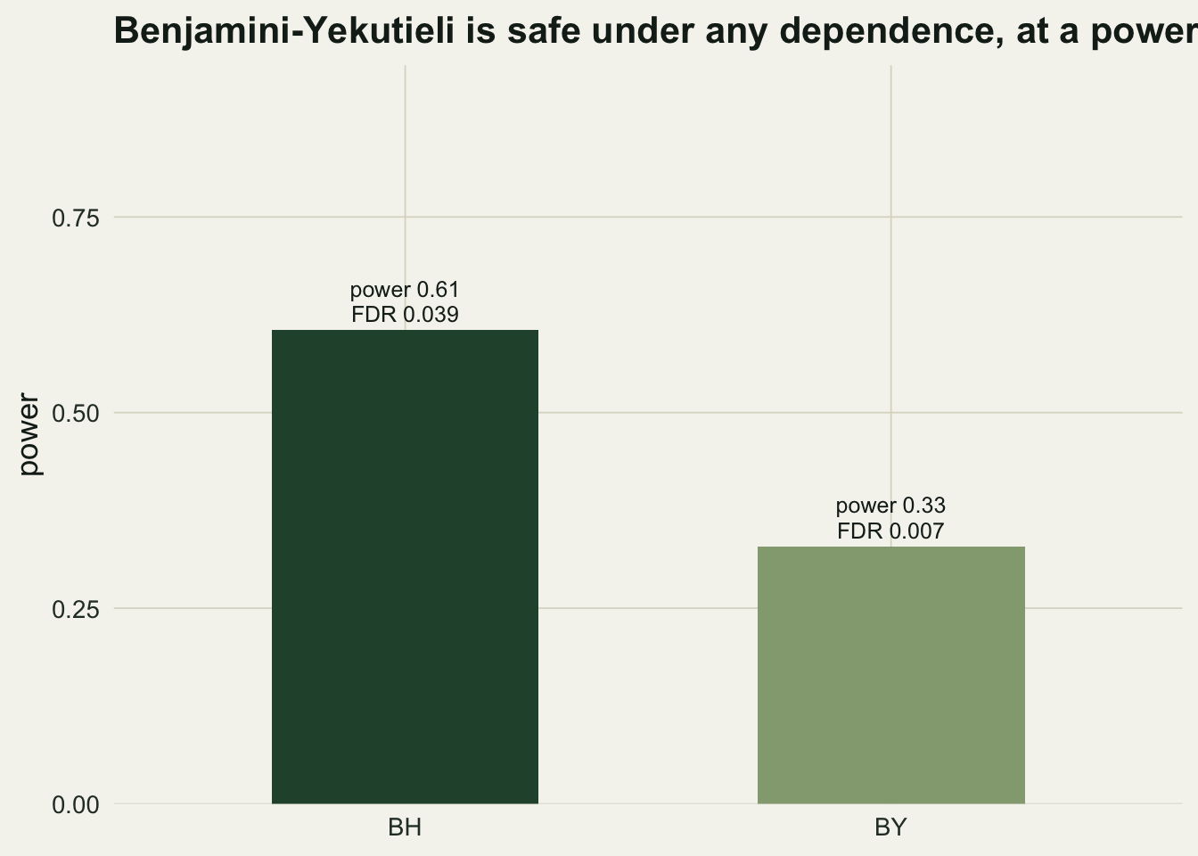
Under independence BY holds the false discovery rate at `r round(res["fdr_by"],4)`, far below the target, and its power is `r round(res["power_by"],3)` against BH's `r round(res["power_bh"],3)`: roughly `r round(res["power_by"]/res["power_bh"],2)` of the detections. That is the trade. BY protects you when the dependence is unknown or adversarial, but if your tests really are independent or positively dependent, it leaves a lot of real signal on the table.
```{r}
#| label: fig-power-fdr
#| fig-cap: "Power and false discovery rate for Benjamini-Hochberg and Benjamini-Yekutieli under independence. BY is safe under any dependence but detects about half as many true effects."
#| fig-alt: "Two bars of power: BH at 0.61, BY at 0.33, each annotated with its false discovery rate of 0.04 and 0.01 respectively."
#| fig-width: 8.5
db <- data.frame(method = factor(c("BH","BY"), levels = c("BH","BY")),
  power = c(res["power_bh"], res["power_by"]),
  fdr   = c(mean(fdp_ind), res["fdr_by"]))
ggplot(db, aes(method, power, fill = method)) +
  geom_col(width = .55) +
  geom_text(aes(label = sprintf("power %.2f\nFDR %.3f", power, fdr)),
            vjust = -0.2, size = 3.3, colour = te_ink, lineheight = .95) +
  scale_fill_manual(values = c(c_bh, c_by), guide = "none") +
  scale_y_continuous(limits = c(0, 0.8), expand = expansion(mult = c(0, .18))) +
  labs(x = NULL, y = "power",
       title = "Benjamini-Yekutieli is safe under any dependence, at a power cost") +
  theme_te() + theme(plot.title.position = "plot")
```
## The honest limit
Which correction is right depends on the dependence structure, and that is the part you cannot see. The p-values alone do not reveal whether the tests are independent, positively dependent, or something worse; PRDS is an assumption about the joint distribution of the statistics, argued from how the data were generated, not read off the output. If you can defend positive dependence, BH is efficient and its rate holds. If you cannot, BY is the honest default, bought at a real cost in power. Either way, the dependence between your tests is external information you bring to the analysis, in the same way that a missingness mechanism or a measurement-error variance has to come from outside the data that exhibit it. The [final tutorial in this series](../checking-a-multiple-testing-analysis/) turns to what you can actually check.
## References
Benjamini Y, Yekutieli D 2001. Ann Stat 29(4):1165-1188 (10.1214/aos/1013699998).
Benjamini Y, Hochberg Y 1995. J R Stat Soc Ser B 57(1):289-300 (10.1111/j.2517-6161.1995.tb02031.x).
Benjamini Y, Krieger AM, Yekutieli D 2006. Biometrika 93(3):491-507 (10.1093/biomet/93.3.491).
Reiner A, Yekutieli D, Benjamini Y 2003. Bioinformatics 19(3):368-375 (10.1093/bioinformatics/btf877).
Efron B 2007. J Am Stat Assoc 102(477):93-103 (10.1198/016214506000001211).
## Related tutorials
- [The false discovery rate and Benjamini-Hochberg](../false-discovery-rate-benjamini-hochberg/)
- [Family-wise error and the Bonferroni correction](../family-wise-error-and-bonferroni/)
- [Checking a multiple-testing analysis](../checking-a-multiple-testing-analysis/)
- [Spatial autocorrelation and Moran's I](../spatial-autocorrelation-morans-i/)