---
title: "Approximate Bayesian computation from scratch"
description: "Fitting an ecological model you can simulate but cannot write a likelihood for. Rejection ABC by hand in R, and the exact price the tolerance charges."
date: "2026-06-14 09:00"
date-modified: "2026-10-15"
categories: [R, approximate Bayesian computation, simulation, ecology tutorial]
image: thumbnail.png
image-alt: "Three overlaid posterior densities of a mean, tightening towards an exact reference curve as the ABC tolerance shrinks."
---
*Corrected 15 October 2026: the section on what the tolerance costs gave its equation for the posterior spread without saying that it is an approximation; it now says that the equation treats the uniform error as normal, which is exact only under a flat prior.*
Most of the models on this blog share a property that is easy to miss because it is so convenient: you can write down the probability of the data. Once you have that, everything follows. `optim` finds the maximum, the Hessian gives standard errors, MCMC explores the posterior.
Plenty of ecological models do not have that property. An individual-based forest model, a stochastic population model observed through counting error, a coalescent genealogy: you can *run* these forwards all day, but the probability of your particular dataset is an integral over every unobserved path the simulator could have taken, and nobody can do that integral.
Approximate Bayesian computation is the response. It replaces "evaluate the likelihood at this parameter" with "simulate at this parameter and see whether the result looks like the data". That sounds like a hack. It is not: done one particular way it is exactly correct, and the whole subject is about what you give up when you leave that way behind. This post builds rejection ABC by hand, checks it against a posterior we can compute in closed form, and then puts it on a model where no closed form exists.
```{r setup}
#| echo: false
#| message: false
#| warning: false
library(ggplot2)
te_ink <- "#16241d"; te_forest <- "#275139"; te_sage <- "#93a87f"
te_paper <- "#f5f4ee"; te_line <- "#dad9ca"; te_rust <- "#b5534e"
te_gold <- "#c9b458"; te_muted <- "#5d6b61"
theme_te <- function(base_size = 11) {
theme_minimal(base_size = base_size) +
theme(panel.grid.minor = element_blank(),
panel.grid.major = element_line(colour = te_line, linewidth = 0.3),
axis.title = element_text(colour = te_muted, size = rel(0.9)),
plot.title = element_text(colour = te_ink, face = "bold", size = rel(1.0)),
plot.subtitle = element_text(colour = te_muted, size = rel(0.85)),
legend.title = element_text(colour = te_muted, size = rel(0.85)),
plot.background = element_rect(fill = "#f5f4ee", colour = NA),
panel.background = element_rect(fill = "#f5f4ee", colour = NA))
}
theme_set(theme_te())
```
## Matching exactly: ABC is not an approximation
Start where the answer is known. Twenty seeds are sown, `r 13` germinate, and we want the posterior for the germination probability under a flat Beta(1, 1) prior. Conjugacy gives Beta(14, 8) and we are done in one line. Pretend we are not.
The ABC algorithm in its oldest form is three lines: draw a parameter from the prior, simulate a dataset at that parameter, keep the parameter if the simulated dataset equals the observed one.
```{r act1}
set.seed(288)
n_trial <- 20L; y_obs <- 13L; M1 <- 400000L

p_prior <- runif(M1)                       # draw from the Beta(1, 1) prior
y_sim   <- rbinom(M1, n_trial, p_prior)    # run the model forwards
p_acc   <- p_prior[y_sim == y_obs]         # keep the exact matches

length(p_acc)
```
```{r act1-check}
acc_rate  <- length(p_acc) / M1
acc_theor <- 1 / (n_trial + 1)
post_m    <- mean(p_acc);  exact_m  <- 14 / 22
post_s    <- sd(p_acc);    exact_s  <- sqrt(14 * 8 / (22^2 * 23))
ks        <- suppressWarnings(ks.test(p_acc, "pbeta", 14, 8))
round(c(acc_rate = acc_rate, acc_theory = acc_theor,
        abc_mean = post_m, exact_mean = exact_m,
        abc_sd = post_s, exact_sd = exact_s, ks_p = ks$p.value), 4)
```
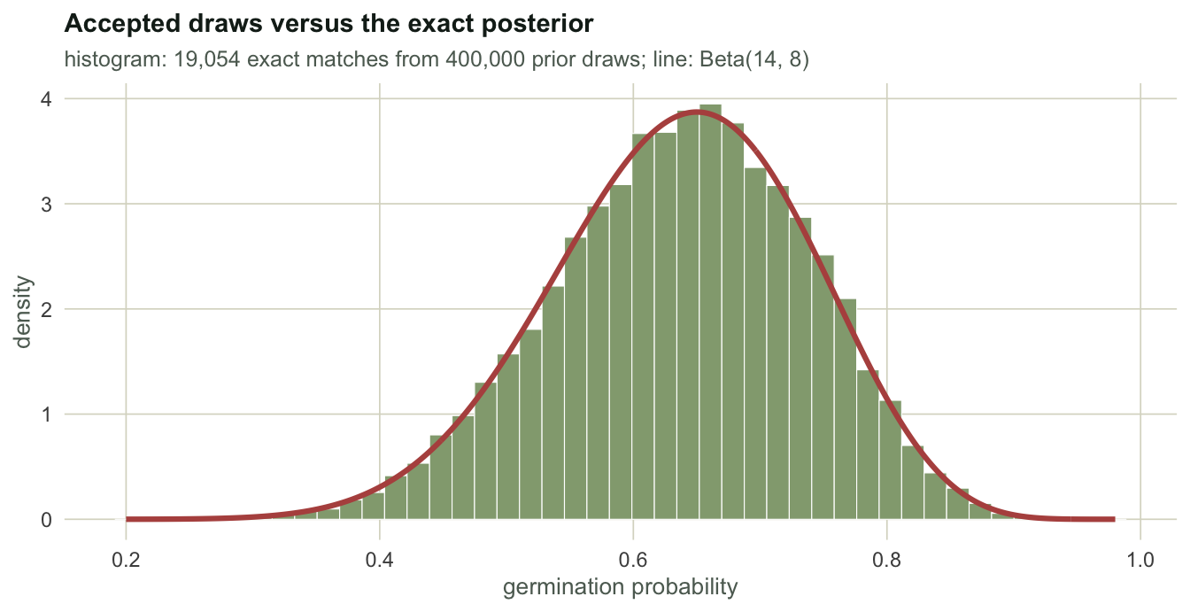
Those `r format(length(p_acc), big.mark = ",")` accepted values are not approximate draws from the posterior. They *are* draws from the posterior, in the same sense that any rejection sampler produces exact draws. The one-line proof: the probability of proposing $p$ and then matching is $\pi(p) \times P(y^\ast = y \mid p)$, which is the prior times the likelihood, which is the posterior up to the constant that rejection sampling throws away for free.
Two numbers confirm it. The Kolmogorov-Smirnov test against Beta(14, 8) gives p = `r round(ks$p.value, 3)`, and the acceptance rate is `r round(acc_rate, 5)` against a theoretical `r round(acc_theor, 5)`. That second one is worth a moment. Under a uniform prior the acceptance rate is $\int \binom{n}{y} p^y (1-p)^{n-y}\,dp = 1/(n+1)$ exactly, whatever `y` happens to be: `r round(acc_theor, 5)` here. It does not depend on the data at all, only on how much data there is. Twenty trials cost you a factor of 21. Two hundred trials would cost a factor of 201, and two hundred *continuous* measurements would cost you everything, which is the next section.
```{r fig-act1}
#| echo: false
#| fig-cap: "Exact-match ABC against the closed-form posterior. The histogram is the accepted prior draws; the line is Beta(14, 8). No tolerance, no summary statistic, no approximation."
#| fig-alt: "Histogram of accepted parameter values with a smooth Beta density curve drawn over it. The curve sits on the histogram across the whole plotted range, roughly 0.2 to 0.95."
#| fig-width: 7
#| fig-height: 3.6
gx <- seq(0.2, 0.98, length.out = 400)
ggplot(data.frame(p = p_acc), aes(p)) +
geom_histogram(aes(y = after_stat(density)), bins = 45,
fill = te_sage, colour = "white", linewidth = 0.2) +
geom_line(data = data.frame(x = gx, y = dbeta(gx, 14, 8)),
aes(x, y), colour = te_rust, linewidth = 1.1, inherit.aes = FALSE) +
labs(x = "germination probability", y = "density",
title = "Accepted draws versus the exact posterior",
subtitle = sprintf("histogram: %s exact matches from %s prior draws; line: Beta(14, 8)",
format(length(p_acc), big.mark = ","), format(M1, big.mark = ",")))
```
## Where the approximation actually enters
Now measure something continuous. Twenty-five plants, each height a draw from a normal with unknown mean and a standard deviation of 1 that we happen to know. The prior on the mean is normal with a standard deviation of `r 10`, wide enough to be nearly flat over anything plausible.
The exact-match rule is now useless: the probability that a simulated dataset reproduces `r 25` real numbers to the last decimal is zero. Two changes rescue it, and they are the only two approximations in all of ABC.
First, compare **summaries** instead of raw data. Here the sample mean is sufficient, so nothing is lost by that step (the next post is about what happens when nothing is not what you lose). Second, accept when the summaries are **close** rather than identical: $|S^\ast - S_{\text{obs}}| < \varepsilon$.
```{r act2-setup}
set.seed(2288)
n <- 25L; sigma_known <- 1; prior_sd <- 10
se <- sigma_known / sqrt(n)                # sampling sd of the summary
y_data <- rnorm(n, mean = 2.0, sd = sigma_known)
s_obs  <- mean(y_data)

# the conjugate answer, for grading
post_prec <- 1 / prior_sd^2 + n / sigma_known^2
post_mean <- (n * s_obs / sigma_known^2) / post_prec
post_sd   <- 1 / sqrt(post_prec)
round(c(s_obs = s_obs, exact_mean = post_mean, exact_sd = post_sd), 4)
```
```{r act2-abc}
M2 <- 2000000L
mu_prior <- rnorm(M2, 0, prior_sd)
s_sim    <- rnorm(M2, mu_prior, se)        # the summary of a simulated dataset
d        <- abs(s_sim - s_obs)

eps_grid <- c(0.02, 0.05, 0.1, 0.2, 0.5, 1.0, 2.0)
sweep_tab <- do.call(rbind, lapply(eps_grid, function(e) {
  keep <- mu_prior[d < e]
  data.frame(eps = e, n_acc = length(keep), rate = length(keep) / M2,
             abc_mean = mean(keep), abc_sd = sd(keep),
             predicted_sd = sqrt(1 / (1 / prior_sd^2 + 1 / (se^2 + e^2 / 3))))
}))
print(sweep_tab, digits = 4, row.names = FALSE)
```
## What the tolerance costs, exactly
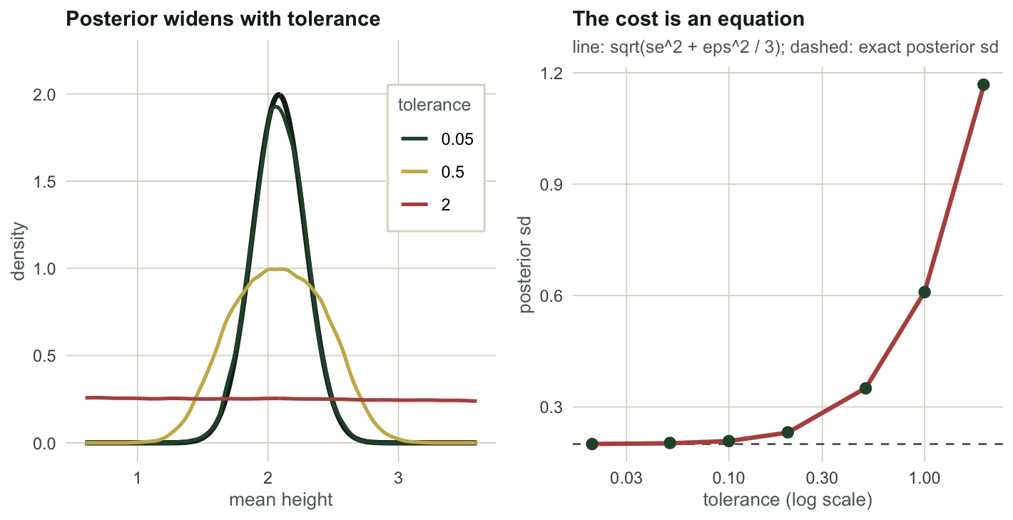
The `predicted_sd` column is not a fudge factor, and it is the reason this example is here rather than a prettier one. Accepting whenever $|S^\ast - S_{\text{obs}}| < \varepsilon$ is the same as saying that the observed summary was generated by the model *and then* shifted by a uniform error on $(-\varepsilon, \varepsilon)$. A uniform on that interval has variance $\varepsilon^2/3$. So ABC with a uniform kernel does not fit your model: it fits your model plus one extra layer of made-up noise, and the posterior inherits the variance of that noise.
```{r act2-cost}
tol_cost <- within(sweep_tab, {
  sd_ratio  <- abc_sd / post_sd
  rel_error <- abs(abc_sd - predicted_sd) / predicted_sd
})
print(tol_cost[, c("eps", "rate", "abc_sd", "predicted_sd", "rel_error", "sd_ratio")],
      digits = 3, row.names = FALSE)
```
The prediction lands to within `r sprintf("%.2f%%", 100 * max(tol_cost$rel_error))` across a hundredfold range of tolerance, which means the cost is not a vague warning but an equation you can solve before you start. The equation is a close approximation rather than an identity: it combines the prior with the sampling variance of the summary and the variance of the uniform error as if that error were normal, which is exact only under a flat prior. At `r sweep_tab$eps[2]` the posterior is `r sprintf("%.0f%%", 100 * (tol_cost$sd_ratio[2] - 1))` wider than the truth and `r sprintf("%.2f%%", 100 * sweep_tab$rate[2])` of proposals survive. At `r sweep_tab$eps[7]` the posterior is `r sprintf("%.1f", tol_cost$sd_ratio[7])` times too wide and `r sprintf("%.0f%%", 100 * sweep_tab$rate[7])` survive. There is no setting that is generous with both.
```{r fig-act2}
#| echo: false
#| fig-cap: "The tolerance is a variance. Left: ABC posteriors at three tolerances against the conjugate answer (black). Right: posterior standard deviation against tolerance, with the predicted curve (the prior combined with a summary variance of se^2 + eps^2 / 3) drawn through the simulated points."
#| fig-alt: "Two panels. On the left, three coloured density curves for the mean; the tightest sits exactly on a black reference curve, the middle one is clearly wider and about half as tall, the widest is a low flat mound. On the right, points rise from a flat floor near 0.2 and turn upwards, with a line passing through every point."
#| fig-width: 7.4
#| fig-height: 3.8
show_eps <- c(0.05, 0.5, 2.0)
dens_df <- do.call(rbind, lapply(show_eps, function(e) {
k <- mu_prior[d < e]
dd <- density(k, n = 512, from = 0.6, to = 3.6)
data.frame(x = dd$x, y = dd$y, eps = factor(e, levels = show_eps))
}))
gx2 <- seq(0.6, 3.6, length.out = 512)
exact_df <- data.frame(x = gx2, y = dnorm(gx2, post_mean, post_sd))
p_left <- ggplot(dens_df, aes(x, y, colour = eps)) +
geom_line(data = exact_df, aes(x, y), colour = te_ink,
linewidth = 1.3, inherit.aes = FALSE) +
geom_line(linewidth = 0.9) +
scale_colour_manual(values = c("0.05" = te_forest, "0.5" = te_gold, "2" = te_rust),
name = "tolerance") +
coord_cartesian(ylim = c(0, 2.2)) +
labs(x = "mean height", y = "density", title = "Posterior widens with tolerance") +
theme(legend.position = "inside", legend.position.inside = c(0.86, 0.72),
legend.background = element_rect(fill = "white", colour = te_line))
p_right <- ggplot(sweep_tab, aes(eps, abc_sd)) +
geom_hline(yintercept = post_sd, linetype = "dashed", colour = te_muted) +
geom_line(aes(y = predicted_sd), colour = te_rust, linewidth = 1.1) +
geom_point(colour = te_forest, size = 2.4) +
scale_x_log10() +
labs(x = "tolerance (log scale)", y = "posterior sd",
title = "The cost is an equation",
subtitle = "line: predicted sd; dashed: exact posterior sd")
grid::grid.newpage()
grid::pushViewport(grid::viewport(layout = grid::grid.layout(1, 2)))
print(p_left, vp = grid::viewport(layout.pos.row = 1, layout.pos.col = 1))
print(p_right, vp = grid::viewport(layout.pos.row = 1, layout.pos.col = 2))
```
Notice also what the acceptance rate does in that table: it roughly doubles when the tolerance doubles. In one summary dimension the acceptance rate scales like $\varepsilon$, so halving the standard deviation of the extra noise is only twice as expensive (halving its variance costs a factor of sqrt(2)). That linear exchange rate is the friendliest ABC ever gets, and it holds only for one summary. With `k` summaries the acceptance region is a ball of radius $\varepsilon$ in `k` dimensions and its volume scales like $\varepsilon^k$.
## A model with no likelihood
Time to earn the machinery. The Ricker map with process noise and Poisson counts (the noisy version is a standard test case for likelihood-free methods: Wood 2010) is:
$$N_t = N_{t-1}\,\exp\!\big(r - N_{t-1} + e_t\big), \qquad e_t \sim N(0, \sigma^2), \qquad y_t \sim \text{Poisson}(\phi N_t)$$
The counts `y` are all you see. The population `N` is latent, the noise `e` is latent, and the likelihood of a fifty-year count series is a fifty-dimensional integral over both. There is no closed form. A particle filter could estimate it, but nothing writes it down. One naming point before the code: the growth term `r` in the equation above is called `log_r` in the code and in the next post, because the Ricker is more often written with the growth rate multiplying from outside the exponential, and this `r` is the log of that.
Simulating it, on the other hand, is a short loop over time. Vectorise across proposals rather than looping over them one at a time and a hundred thousand simulated ecosystems take under a second.
```{r ricker-sim}
sim_ricker <- function(log_r, sigma, phi, n, N0 = 1) {
  M <- length(log_r)
  N <- rep(N0, M)
  Y <- matrix(0L, M, n)
  for (t in 1:n) {                          # loop over TIME, not over proposals
    N <- N * exp(log_r - N + rnorm(M, 0, sigma))
    Y[, t] <- rpois(M, phi * N)
  }
  Y
}

summ <- function(Y) {                       # three summaries per simulated series
  m   <- rowMeans(Y)
  sdv <- sqrt(rowMeans(Y^2) - m^2) * sqrt(ncol(Y) / (ncol(Y) - 1))
  Yc  <- Y - m
  a1  <- rowSums(Yc[, -1, drop = FALSE] * Yc[, -ncol(Y), drop = FALSE]) / rowSums(Yc^2)
  cbind(mean = m, cv = sdv / pmax(m, 1e-8), acf1 = a1)
}
```
```{r ricker-data}
set.seed(3288)
true_log_r <- 1.5; true_sigma <- 0.3; phi_known <- 20; nyr <- 50L
y_ric <- as.vector(sim_ricker(true_log_r, true_sigma, phi_known, nyr))
S_obs <- summ(matrix(y_ric, nrow = 1))
round(S_obs, 4)
```
Those three summaries come from what the model is made of, not from a menu. The mean count tracks the equilibrium, which for this map is $N^\ast = r$: the observed series gives `r round(mean(y_ric) / phi_known, 2)` against a true `r true_log_r`. The coefficient of variation carries the process noise sitting on top of the Poisson noise. And the lag-1 autocorrelation reads the return rate of the map, which the linearisation puts at $1 - N^\ast$, or `r 1 - true_log_r` here, and which goes negative once density dependence overcompensates. That last summary lands at `r round(S_obs[3], 2)` rather than `r 1 - true_log_r`, for two reasons worth knowing: the linearisation only holds for small noise, and the Poisson layer piles uncorrelated variance on top, pulling the correlation towards zero exactly as [measurement error attenuates a regression slope](../measurement-error-regression-dilution/).
The distance needs one more decision. The three summaries live on wildly different scales (counts around `r round(S_obs[1])`, a ratio near `r round(S_obs[2], 2)`, a correlation near `r round(S_obs[3], 2)`), so a raw Euclidean distance would spend almost its whole budget matching the mean count and let the other two drift. Divide each summary by its spread across the prior draws first, which is what the standard implementations do (Beaumont 2002); the [next post](../summary-statistics-for-abc/) measures what happens if you do not.
```{r ricker-abc}
set.seed(4288)
M3 <- 200000L
th_lr <- runif(M3, 0, 3)                    # prior on r
th_sg <- runif(M3, 0, 1)                    # prior on sigma
S <- summ(sim_ricker(th_lr, th_sg, phi_known, nyr))

scale_S <- apply(S, 2, mad)                 # spread under the prior predictive
Z    <- sweep(sweep(S, 2, as.vector(S_obs), "-"), 2, scale_S, "/")
dist <- sqrt(rowSums(Z^2))

keep_frac <- 0.0025                         # keep the closest 0.25 per cent
tol  <- unname(quantile(dist, keep_frac))
sel  <- dist <= tol
post <- data.frame(log_r = th_lr[sel], sigma = th_sg[sel])
c(kept = nrow(post), tolerance = round(tol, 4))
```
```{r ricker-summary}
ci <- function(x) round(c(mean = mean(x), quantile(x, c(0.025, 0.975))), 3)
rbind(log_r = ci(post$log_r), sigma = ci(post$sigma))
```
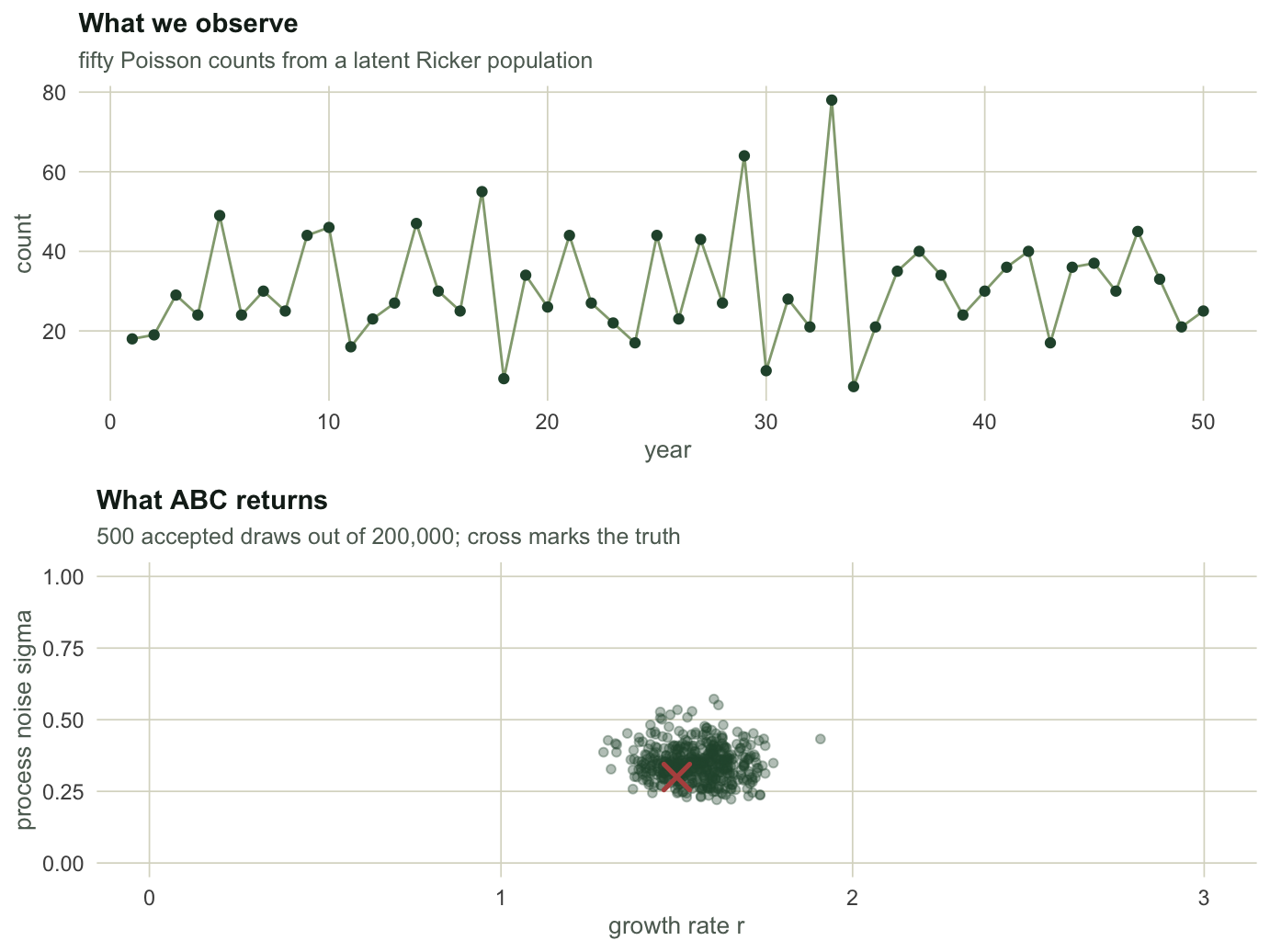
The posterior mean for the growth rate is `r round(mean(post$log_r), 3)` against a truth of `r true_log_r`, with a 95 per cent credible interval of `r sprintf("[%.2f, %.2f]", quantile(post$log_r, 0.025), quantile(post$log_r, 0.975))`. For the process noise it is `r round(mean(post$sigma), 3)` against `r true_sigma`, interval `r sprintf("[%.2f, %.2f]", quantile(post$sigma, 0.025), quantile(post$sigma, 0.975))`. Both cover, and the two are not trading off against each other: their correlation across the accepted draws is `r sprintf("%.3f", cor(post$log_r, post$sigma))` (p = `r sprintf("%.2f", cor.test(post$log_r, post$sigma)$p.value)`), so the mean count is doing the work for one parameter and the variability for the other. We never wrote a likelihood, and the only R functions involved were `runif`, `rnorm`, `rpois`, `mad` and `quantile`.
```{r fig-ricker}
#| echo: false
#| fig-cap: "Fitting the stochastic Ricker with no likelihood. Top: the fifty counts that are all we observe. Bottom: the 500 accepted parameter pairs, with the truth as a cross. The cloud takes a wider share of the noise axis than of the growth axis, and it does not tilt: these summaries separate the two parameters rather than trading them off."
#| fig-alt: "Top panel shows a jagged count series swinging between single digits and the high seventies across fifty years, with no drift up or down. Bottom panel is a scatter of accepted parameter pairs forming a loose untilted cloud, taking a wider share of the noise axis than of the growth axis, with a cross marking the true values inside it."
#| fig-width: 7.2
#| fig-height: 5.4
p_ts <- ggplot(data.frame(t = seq_len(nyr), y = y_ric), aes(t, y)) +
geom_line(colour = te_sage, linewidth = 0.5) +
geom_point(colour = te_forest, size = 1.5) +
labs(x = "year", y = "count", title = "What we observe",
subtitle = "fifty Poisson counts from a latent Ricker population")
p_sc <- ggplot(post, aes(log_r, sigma)) +
geom_point(colour = te_forest, alpha = 0.35, size = 1.4) +
annotate("point", x = true_log_r, y = true_sigma, shape = 4,
size = 4, stroke = 1.4, colour = te_rust) +
coord_cartesian(xlim = c(0, 3), ylim = c(0, 1)) +
labs(x = "growth rate r", y = "process noise sigma",
title = "What ABC returns",
subtitle = sprintf("%s accepted draws out of %s; cross marks the truth",
nrow(post), format(M3, big.mark = ",")))
grid::grid.newpage()
grid::pushViewport(grid::viewport(layout = grid::grid.layout(2, 1)))
print(p_ts, vp = grid::viewport(layout.pos.row = 1, layout.pos.col = 1))
print(p_sc, vp = grid::viewport(layout.pos.row = 2, layout.pos.col = 1))
```
## Where to go next
Look again at what the fit cost: `r format(M3, big.mark = ",")` simulations to buy `r nrow(post)` posterior draws. The other `r sprintf("%.2f%%", 100 * (1 - keep_frac))` of the work went in the bin, because rejection ABC proposes from the prior and the prior is mostly wrong. That waste is the entire reason the rest of this cluster exists, and it splits into two separate complaints that get confused constantly.
The first is statistical. Everything you accept is filtered through the summaries and the tolerance, so the thing you sampled is not the posterior given the data: it is the posterior given `r ncol(S)` numbers, blurred by a uniform kernel. More simulations will not fix either. Where those `r ncol(S)` numbers came from, and what it costs to pick them badly, is the subject of the [next post](../summary-statistics-for-abc/).
The second is computational. The eps-posterior you settled for is a fixed target, and rejection sampling is simply a bad way to hit it. Proposing from the prior means proposing mostly into regions the data have already ruled out, and [ABC-MCMC and sequential ABC](../abc-mcmc-and-sequential-abc/) both fix that by proposing from something better.
Keep the two apart, because they get confused constantly. Better sampling makes the answer cheaper. Only better summaries and smaller tolerances make it more correct.
## References
- Pritchard, Seielstad, Perez-Lezaun, Feldman 1999 Molecular Biology and Evolution 16(12):1791-1798 (10.1093/oxfordjournals.molbev.a026091)
- Beaumont, Zhang, Balding 2002 Genetics 162(4):2025-2035 (10.1093/genetics/162.4.2025)
- Wood 2010 Nature 466(7310):1102-1104 (10.1038/nature09319)
- Beaumont 2010 Annual Review of Ecology, Evolution, and Systematics 41(1):379-406 (10.1146/annurev-ecolsys-102209-144621)
- Csillery, Blum, Gaggiotti, Francois 2010 Trends in Ecology and Evolution 25:410-418 (10.1016/j.tree.2010.04.001)
- Fearnhead, Prangle 2012 Journal of the Royal Statistical Society B 74(3):419-474 (10.1111/j.1467-9868.2011.01010.x)
- Blum, Nunes, Prangle, Sisson 2013 Statistical Science 28(2):189-208 (10.1214/12-STS406)
## Related tutorials
- [Choosing summary statistics for ABC](../summary-statistics-for-abc/)
- [Metropolis-Hastings from scratch](../metropolis-hastings-from-scratch/)
- [The parametric bootstrap](../the-parametric-bootstrap/)
- [ABC-MCMC and sequential ABC samplers](../abc-mcmc-and-sequential-abc/)