Choosing summary statistics for ABC

In ABC the summaries are the data. Sufficiency, the price of a useless summary, distance scaling and semi-automatic ABC, measured in R on a Ricker model.

Rejection ABC accepts a proposal when the simulated summaries land close enough to the observed ones. The previous post spent its effort on “close enough” and showed that the tolerance adds a known, controllable variance. It quietly made two other decisions and defended neither: it picked three summaries for the Ricker model out of the dozens available, and it divided each of them by a scale factor before measuring distance.

Those two decisions do more to the answer than the tolerance does, and unlike the tolerance they do not go away when you buy more computer. This post measures both, and then hands the job to a regression.

library(ggplot2)

te_ink <- "#16241d"; te_forest <- "#275139"; te_sage <- "#93a87f"
te_paper <- "#f5f4ee"; te_line <- "#dad9ca"; te_rust <- "#b5534e"
te_gold <- "#c9b458"; te_muted <- "#5d6b61"

theme_te <- function(base_size = 12) {
  theme_minimal(base_size = base_size) +
    theme(panel.grid.minor = element_blank(),
          panel.grid.major = element_line(colour = te_line, linewidth = 0.3),
          plot.title = element_text(colour = te_ink, face = "bold"),
          plot.subtitle = element_text(colour = te_muted, size = rel(0.85)),
          axis.title = element_text(colour = te_muted),
          axis.text = element_text(colour = te_muted),
          strip.text = element_text(colour = te_ink, face = "bold"),
          legend.title = element_text(colour = te_muted, size = rel(0.85)))
}
theme_set(theme_te())

What a summary throws away is gone for good

The clean way to see this is a problem where the exact posterior is available, so that every gap has a name. Twenty-five draws from a normal with a known standard deviation of 1, an unknown mean, and a wide normal prior. The sample mean is sufficient: it carries every scrap of information the data hold about the mean. The sample median is not, though it is a perfectly sensible estimator that most ecologists would trust on sight.

set.seed(289)
n_s <- 25L; sig_s <- 1; prior_sd_s <- 10
y_s <- rnorm(n_s, 2.0, sig_s)
mean_obs <- mean(y_s); med_obs <- median(y_s)

post_prec <- 1 / prior_sd_s^2 + n_s / sig_s^2
exact_mean <- (n_s * mean_obs / sig_s^2) / post_prec
exact_sd   <- 1 / sqrt(post_prec)
c(mean_obs = mean_obs, med_obs = med_obs, exact_sd = exact_sd)

mean_obs  med_obs exact_sd 
2.029159 2.045334 0.199960 

Now run rejection ABC twice on the same simulations, once matching the mean and once matching the median. Every proposal generates a full data set of 25 numbers, and both summaries are read off it, so the two runs differ in nothing but the summary they compare.

M_s <- 400000L
mu_s <- rnorm(M_s, 0, prior_sd_s)
X_s  <- matrix(rnorm(M_s * n_s, rep(mu_s, n_s), sig_s), M_s, n_s)
s_mean <- rowMeans(X_s)
s_med  <- apply(X_s, 1, median)

keep_q <- function(d, q = 0.005) d <= quantile(d, q)
acc_mean <- keep_q(abs(s_mean - mean_obs))
acc_med  <- keep_q(abs(s_med  - med_obs))
c(n_accepted = sum(acc_mean),
  sd_from_mean = sd(mu_s[acc_mean]),
  sd_from_median = sd(mu_s[acc_med]))

    n_accepted   sd_from_mean sd_from_median 
  2000.0000000      0.2060681      0.2533884 

gx <- seq(exact_mean - 4 * exact_sd, exact_mean + 4 * exact_sd, length.out = 512)
dens_s <- rbind(
  data.frame(x = density(mu_s[acc_mean], n = 512, from = min(gx), to = max(gx))$x,
             y = density(mu_s[acc_mean], n = 512, from = min(gx), to = max(gx))$y,
             src = "sample mean (sufficient)"),
  data.frame(x = density(mu_s[acc_med], n = 512, from = min(gx), to = max(gx))$x,
             y = density(mu_s[acc_med], n = 512, from = min(gx), to = max(gx))$y,
             src = "sample median (not)"))

ggplot(dens_s, aes(x, y, colour = src)) +
  geom_line(data = data.frame(x = gx, y = dnorm(gx, exact_mean, exact_sd)),
            aes(x, y), colour = te_ink, linewidth = 1.4, inherit.aes = FALSE) +
  geom_line(linewidth = 1) +
  scale_colour_manual(values = c("sample mean (sufficient)" = te_forest,
                                 "sample median (not)" = te_rust), name = NULL) +
  labs(title = "The summary sets the floor, not the tolerance",
       subtitle = "black: exact posterior; coloured: ABC posteriors at the same tolerance quantile",
       x = "mean", y = "density") +
  theme(legend.position = c(0.8, 0.8),
        legend.background = element_rect(fill = te_paper, colour = NA))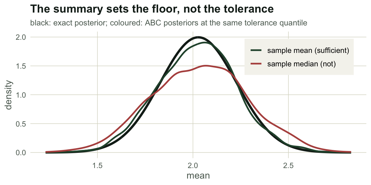

Figure 1: Rejection ABC on the same 400,000 simulations, differing only in which summary is compared. The sufficient summary recovers the exact posterior; the median throws away a fixed share of the information and no tolerance brings it back.

The median-based posterior is 1.23 times wider. That number is not an ABC artefact, and this is the part worth internalising: it is the median’s own inefficiency, showing through. Across these same simulations the sample median of 25 normal draws has a standard deviation of 0.2487 around the true mean against the sample mean’s 0.2, a ratio of 1.244, heading for \(\sqrt{\pi/2} = 1.2533\) as the sample grows.

ABC reproduces that ratio and nothing more. The tolerance error shrinks to nothing as you tighten it; the summary error does not shrink at all. A million more simulations buy you a better estimate of the wrong posterior.

What a useless summary costs

Sufficiency argues for keeping more summaries. Reality argues back. Take the same problem, keep the sufficient summary, and add summaries that carry literally nothing: independent standard normal draws, unrelated to the parameter and unrelated to the data. Then accept a fixed number of draws, so the simulation budget never changes.

set.seed(2289)
M_d <- 600000L; K <- 10L; n_keep <- 2000L
mu_d <- rnorm(M_d, 0, prior_sd_s)
s1   <- rnorm(M_d, mu_d, sig_s / sqrt(n_s))
NZ   <- matrix(rnorm(M_d * K), M_d, K)
nz_obs <- rnorm(K)

sweep_k <- data.frame(k = c(0L, 1L, 2L, 3L, 5L, 10L))
sweep_k$abc_sd <- NA_real_; sweep_k$tol_s1 <- NA_real_; sweep_k$keep <- vector("list", nrow(sweep_k))
for (i in seq_len(nrow(sweep_k))) {
  k  <- sweep_k$k[i]
  d2 <- (s1 - mean_obs)^2
  if (k > 0) {
    j  <- seq_len(k)
    d2 <- d2 + rowSums(sweep(NZ[, j, drop = FALSE], 2, nz_obs[j], "-")^2)
  }
  d   <- sqrt(d2)
  sel <- d <= sort(d, partial = n_keep)[n_keep]
  sweep_k$abc_sd[i] <- sd(mu_d[sel])
  sweep_k$tol_s1[i] <- max(abs(s1[sel] - mean_obs))
  sweep_k$keep[[i]] <- mu_d[sel]
}
sweep_k$widening <- sweep_k$abc_sd / exact_sd
print(sweep_k[, c("k", "abc_sd", "tol_s1", "widening")], digits = 3)

   k abc_sd tol_s1 widening
1  0  0.200 0.0439     1.00
2  1  0.239 0.2668     1.19
3  2  0.350 0.6297     1.75
4  3  0.420 0.8751     2.10
5  5  0.841 2.2682     4.20
6 10  0.974 2.6938     4.87

show_k <- c(0L, 2L, 5L, 10L)
gxd <- seq(exact_mean - 12 * exact_sd, exact_mean + 12 * exact_sd, length.out = 512)
dens_d <- do.call(rbind, lapply(show_k, function(kk) {
  v <- sweep_k$keep[[match(kk, sweep_k$k)]]
  dd <- density(v, n = 512, from = min(gxd), to = max(gxd))
  data.frame(x = dd$x, y = dd$y, k = factor(kk, levels = show_k))
}))

p1 <- ggplot(dens_d, aes(x, y, colour = k)) +
  geom_line(data = data.frame(x = gxd, y = dnorm(gxd, exact_mean, exact_sd)),
            aes(x, y), colour = te_ink, linewidth = 1.2, linetype = "dashed",
            inherit.aes = FALSE) +
  geom_line(linewidth = 1) +
  scale_colour_manual(values = setNames(c(te_forest, te_sage, te_gold, te_rust), show_k),
                      name = "noise summaries") +
  labs(title = "Each empty summary widens it", x = "mean", y = "density") +
  theme(legend.position = c(0.83, 0.68),
        legend.background = element_rect(fill = te_paper, colour = NA),
        legend.key.size = unit(0.8, "lines"))

p2 <- ggplot(sweep_k, aes(k, abc_sd)) +
  geom_hline(yintercept = exact_sd, colour = te_ink, linetype = "dashed") +
  geom_line(colour = te_rust, linewidth = 0.9) +
  geom_point(colour = te_forest, size = 2.4) +
  annotate("text", x = 6.2, y = exact_sd * 1.5, label = "exact posterior sd",
           colour = te_ink, size = 3.2, hjust = 0) +
  labs(title = "The cost is not gentle", x = "summaries carrying nothing",
       y = "ABC posterior sd")

gridExtra_free <- function(a, b) {
  grid::grid.newpage()
  grid::pushViewport(grid::viewport(layout = grid::grid.layout(1, 2)))
  print(a, vp = grid::viewport(layout.pos.row = 1, layout.pos.col = 1))
  print(b, vp = grid::viewport(layout.pos.row = 1, layout.pos.col = 2))
}
gridExtra_free(p1, p2)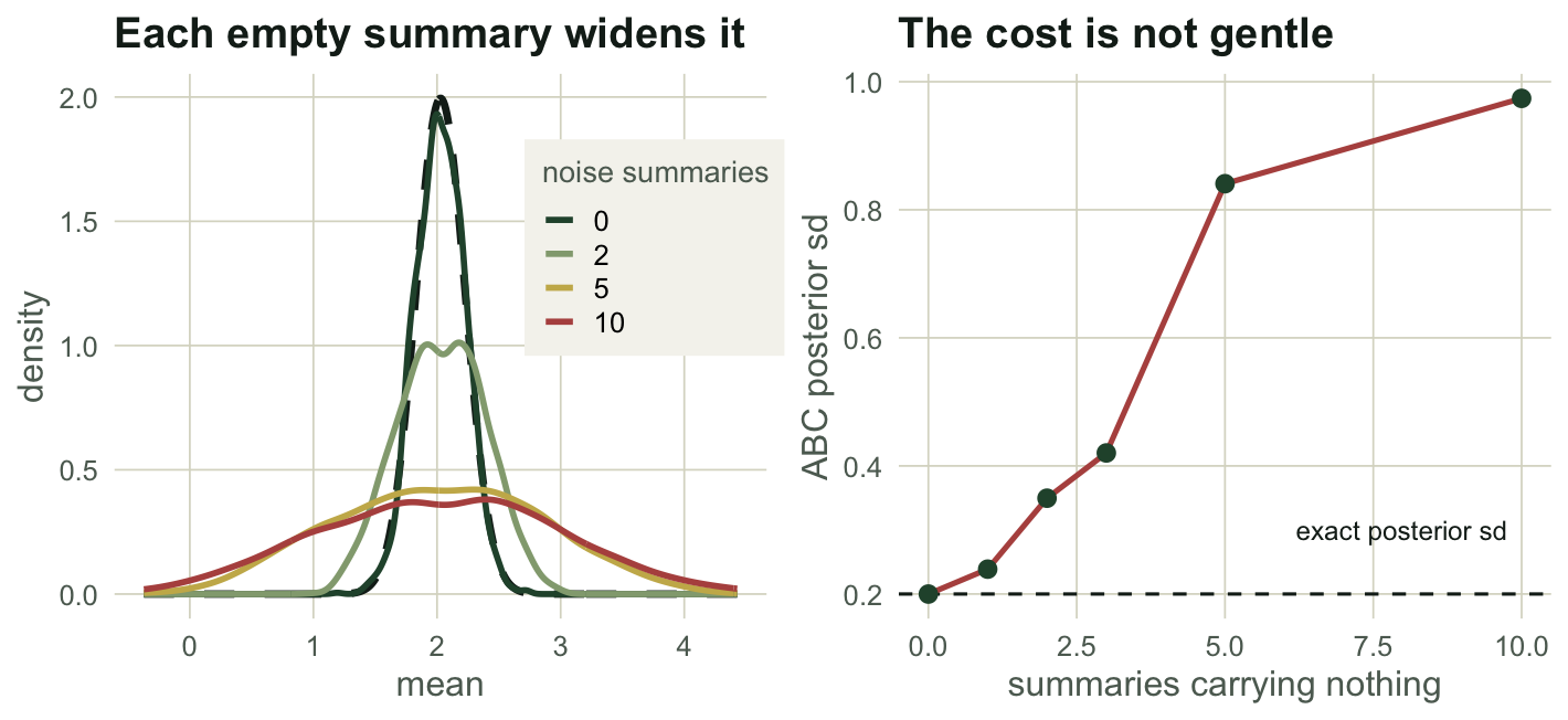

Figure 2: Ten summaries carrying no information at all, added to a distance that already contained a sufficient one. The simulation budget and the number of accepted draws are held fixed, so the only thing that changes is how the tolerance gets spent.

Ten summaries that a coin flip could have produced, and the posterior is 4.9 times wider than the exact one. The mechanism is in the tolerance column: matching the sufficient summary to within 0.044 when it stands alone, the same acceptance count forces it out to 2.69 once ten passengers ride along.

The geometry is worth a sentence. To keep a fixed fraction \(q\) of the draws inside a ball in \(d\) dimensions, the radius has to grow like \(q^{1/d}\), because the volume goes like \(r^d\). A one-in-300 cut is a tight interval on one axis and a comfortable stroll on eleven. The accepted set stops meaning “draws that reproduce the data” and starts meaning “draws that struck a decent compromise across eleven axes, ten of which are gibberish”.

So sufficiency and dimension pull in opposite directions, and the whole literature on summary choice lives in that tension (Blum 2013).

The distance is a choice too

Back to the stochastic Ricker from the previous post, with the same three summaries: mean count, coefficient of variation, and lag-1 autocorrelation.

sim_ricker <- function(log_r, sigma, phi, n_years, N0 = 1) {
  M <- length(log_r); N <- rep(N0, M); Y <- matrix(0L, M, n_years)
  for (t in seq_len(n_years)) {
    N <- N * exp(log_r - N + rnorm(M, 0, sigma))
    Y[, t] <- rpois(M, phi * N)
  }
  Y
}

summ8 <- function(Y) {
  nn <- ncol(Y); m <- rowMeans(Y)
  sdv <- sqrt(pmax(rowMeans(Y^2) - m^2, 0)) * sqrt(nn / (nn - 1))
  Yc <- Y - m; den <- pmax(rowSums(Yc^2), 1e-9)
  cbind(mean  = m,
        sd    = sdv,
        cv    = sdv / pmax(m, 1e-8),
        acf1  = rowSums(Yc[, -1, drop = FALSE] * Yc[, -nn, drop = FALSE]) / den,
        acf2  = rowSums(Yc[, -(1:2), drop = FALSE] * Yc[, -((nn - 1):nn), drop = FALSE]) / den,
        max   = apply(Y, 1, max),
        zeros = rowSums(Y == 0),
        jump  = rowMeans(abs(Y[, -1, drop = FALSE] - Y[, -nn, drop = FALSE])))
}

set.seed(3289)
true_lr <- 1.5; true_sg <- 0.3; phi_known <- 20; n_years <- 50L
y_ric <- as.vector(sim_ricker(true_lr, true_sg, phi_known, n_years))
S_obs <- summ8(matrix(y_ric, nrow = 1))
round(S_obs[, c("mean", "cv", "acf1")], 3)

  mean     cv   acf1 
30.520  0.339 -0.351 

set.seed(4289)
M_r <- 200000L
lr <- runif(M_r, 0, 3); sg <- runif(M_r, 0, 1)
S_all <- summ8(sim_ricker(lr, sg, phi_known, n_years))
i3 <- c("mean", "cv", "acf1")
scale3 <- apply(S_all[, i3], 2, mad)
round(scale3, 3)

  mean     cv   acf1 
22.536  0.464  0.311 

There is the problem, in three numbers. The mean count is measured in animals and varies by 22.5 across the prior draws; the coefficient of variation is a ratio and varies by 0.46; the autocorrelation is bounded and varies by 0.31. A raw Euclidean distance treats one animal as interchangeable with 2.2 prior-widths of the coefficient of variation. Nobody decided that. The units did.

Dev  <- sweep(S_all[, i3], 2, S_obs[, i3], "-")
d_raw <- sqrt(rowSums(Dev^2))
d_std <- sqrt(rowSums(sweep(Dev, 2, scale3, "/")^2))
n_acc <- 500L

pick_n <- function(d, k = n_acc) d <= sort(d, partial = k)[k]
a_raw <- pick_n(d_raw); a_std <- pick_n(d_std)

report <- function(sel, label) {
  data.frame(distance = label,
             mean_matched_to = max(abs(Dev[sel, "mean"])),
             cv_lo = min(S_all[sel, "cv"]),  cv_hi = max(S_all[sel, "cv"]),
             sigma_post_sd = sd(sg[sel]),
             sigma_mean = mean(sg[sel]))
}
scale_tab <- rbind(report(a_raw, "raw"), report(a_std, "standardised"))
print(scale_tab, digits = 3, row.names = FALSE)

     distance mean_matched_to cv_lo cv_hi sigma_post_sd sigma_mean
          raw            0.24 0.149 0.584        0.1183      0.259
 standardised            3.42 0.270 0.409        0.0557      0.247

gxs <- seq(0, 1, length.out = 512)
dens_sc <- rbind(
  data.frame(x = density(sg[a_raw], n = 512, from = 0, to = 1)$x,
             y = density(sg[a_raw], n = 512, from = 0, to = 1)$y, d = "raw"),
  data.frame(x = density(sg[a_std], n = 512, from = 0, to = 1)$x,
             y = density(sg[a_std], n = 512, from = 0, to = 1)$y, d = "standardised"))

ggplot(dens_sc, aes(x, y, colour = d)) +
  geom_hline(yintercept = 1, colour = te_muted, linetype = "dotted") +
  geom_vline(xintercept = true_sg, colour = te_ink, linetype = "dashed") +
  geom_line(linewidth = 1) +
  annotate("text", x = 0.88, y = 1.35, label = "prior", colour = te_muted, size = 3.2) +
  annotate("text", x = true_sg, y = 7.4, label = " truth", colour = te_ink,
           size = 3.2, hjust = 0) +
  scale_colour_manual(values = c(raw = te_rust, standardised = te_forest),
                      name = "distance") +
  coord_cartesian(xlim = c(0, 1), ylim = c(0, 7.8), expand = FALSE) +
  labs(title = "Units are not a modelling decision, but they act like one",
       x = "process noise sigma", y = "density") +
  theme(legend.position = c(0.82, 0.62),
        legend.background = element_rect(fill = te_paper, colour = NA))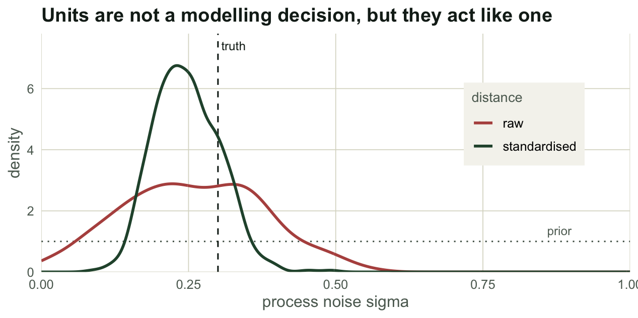

Figure 3: Process-noise posteriors from the same simulations and the same three summaries, under a raw and a scale-corrected Euclidean distance. The flat line is the prior. The raw distance spends its tolerance on the summary with the biggest units, and learns roughly half as much about the parameter that the other two carry.

The raw distance matches the mean count to within 0.24 of a single animal, which is far tighter than the data could ever justify, and pays for that precision by letting the coefficient of variation wander from 0.15 to 0.58. The scale-corrected distance lets the mean count off by up to 3.4 animals and holds the coefficient of variation inside 0.27 to 0.41 instead. The consequence lands on the parameter those shape summaries carry: the process-noise posterior has a standard deviation of 0.118 under the raw distance against 0.056 under the corrected one, out of a prior standard deviation of 0.289.

The raw distance is not exactly wrong. It answers a different question, one chosen for it by whoever decided to count animals rather than record them per hundred hectares. Ecologists have met this before: it is the same argument as choosing a dissimilarity index for community data, where the decision to standardise decides what the ordination is about. Dividing by the median absolute deviation of the prior draws is the usual default (Beaumont 2002), and better distances exist (Prangle 2017).

Letting a regression choose

Here is the awkward position. Sufficiency wants every summary you can think of. Dimension wants almost none. Scaling wants you to have thought about units. And ecological models offer summaries by the dozen: means, variances, autocorrelations at several lags, extremes, zero counts, the average year-on-year jump.

Fearnhead and Prangle (2012) turn this into an estimation problem with a result behind it. If your loss is squared error, the optimal summary for parameter \(\theta_i\) is its posterior mean \(\mathbb{E}[\theta_i \mid \text{data}]\). You do not know that function, but you can regress it: simulate parameters and data sets, then fit \(\theta_i\) against the candidate summaries. The fitted values become your summaries. Two parameters give two summaries, regardless of how many candidates you started from, so the dimension problem simply leaves.

The method has two steps and the first one is the one people skip.

d_pilot <- d_std
box_sel <- pick_n(d_pilot, 2000L)
box <- rbind(log_r = range(lr[box_sel]), sigma = range(sg[box_sel]))
round(box, 3)

       [,1]  [,2]
log_r 1.145 1.913
sigma 0.001 0.508

Step one is a crude pilot run whose only job is to find where the posterior lives, so that the prior can be truncated to that region. Step two fits the regression on simulations from the truncated prior. Why it matters is measurable: over the full prior, which spans everything from collapse to chaos, the relationship between a parameter and any summary is nowhere near a polynomial, and the fit is hopeless.

scale8 <- apply(S_all, 2, mad); scale8[scale8 == 0] <- 1
Z_full <- sweep(S_all, 2, scale8, "/")
B_full <- cbind(1, Z_full, Z_full^2)
h_full <- 1:100000
resid_sd <- function(fit) sqrt(sum(fit$residuals^2) / (length(fit$residuals) - length(fit$coefficients)))
c(full_prior_lr = resid_sd(lm.fit(B_full[h_full, ], lr[h_full])),
  full_prior_sg = resid_sd(lm.fit(B_full[h_full, ], sg[h_full])))

full_prior_lr full_prior_sg 
   0.09590164    0.12140684 

set.seed(6289)
M_t <- 100000L
lr_t <- runif(M_t, box["log_r", 1], box["log_r", 2])
sg_t <- runif(M_t, box["sigma", 1], box["sigma", 2])
S_t  <- summ8(sim_ricker(lr_t, sg_t, phi_known, n_years))

scale_t <- apply(S_t, 2, mad); scale_t[scale_t == 0] <- 1
Z_t  <- sweep(S_t, 2, scale_t, "/")
Zo_t <- S_obs / scale_t
B_t  <- cbind(1, Z_t, Z_t^2)
Bo_t <- cbind(1, Zo_t, Zo_t^2)

fit_half <- 1:50000; abc_half <- 50001:M_t
f_lr <- lm.fit(B_t[fit_half, ], lr_t[fit_half])
f_sg <- lm.fit(B_t[fit_half, ], sg_t[fit_half])
c(truncated_lr = resid_sd(f_lr), truncated_sg = resid_sd(f_sg))

truncated_lr truncated_sg 
  0.05451147   0.04307452 

The pilot region cuts the regression’s residual standard deviation for the process noise from 0.121 to 0.043. That is the whole reason step one exists: the projection only has to be good where the posterior actually is.

Now run three ABC analyses on the identical simulations and the identical budget, differing only in what goes into the distance.

proj <- function(fit, B) as.vector(B %*% fit$coefficients)
P  <- cbind(proj(f_lr, B_t),  proj(f_sg, B_t))
Po <- c(proj(f_lr, Bo_t), proj(f_sg, Bo_t))
scale_P <- apply(P[abc_half, ], 2, mad)

dist_of <- function(Z, Zo, sc) {
  d <- sqrt(rowSums(sweep(sweep(Z, 2, Zo, "-"), 2, sc, "/")^2))
  d[fit_half] <- Inf   # the fitting half is spent; it cannot also be the posterior
  d
}
cands <- list(
  "all 8"        = dist_of(Z_t, as.vector(Zo_t), rep(1, 8)),
  "hand-picked 3"= dist_of(Z_t[, i3], as.vector(Zo_t[, i3]), rep(1, 3)),
  "semi-auto 2"  = dist_of(P, Po, scale_P))

fp_tab <- do.call(rbind, lapply(names(cands), function(nm) {
  sel <- pick_n(cands[[nm]], n_acc)
  data.frame(summaries = nm, log_r_mean = mean(lr_t[sel]), log_r_sd = sd(lr_t[sel]),
             sigma_mean = mean(sg_t[sel]), sigma_sd = sd(sg_t[sel]))
}))
print(fp_tab, digits = 3, row.names = FALSE)

     summaries log_r_mean log_r_sd sigma_mean sigma_sd
         all 8       1.51   0.0845      0.252   0.0514
 hand-picked 3       1.52   0.0657      0.250   0.0477
   semi-auto 2       1.52   0.0569      0.265   0.0439

sel_list <- lapply(cands, pick_n, k = n_acc)
mk <- function(par_vals, lab, from, to) {
  do.call(rbind, lapply(names(sel_list), function(nm) {
    dd <- density(par_vals[sel_list[[nm]]], n = 512, from = from, to = to)
    data.frame(x = dd$x, y = dd$y, summaries = factor(nm, levels = names(cands)), par = lab)
  }))
}
dens_fp <- rbind(mk(lr_t, "growth rate log_r", 1.15, 1.95),
                 mk(sg_t, "process noise sigma", 0, 0.51))
truths  <- data.frame(par = c("growth rate log_r", "process noise sigma"),
                      v = c(true_lr, true_sg))
pal_fp <- c("all 8" = te_rust, "hand-picked 3" = te_gold, "semi-auto 2" = te_forest)

ggplot(dens_fp, aes(x, y, colour = summaries)) +
  geom_vline(data = truths, aes(xintercept = v), colour = te_ink, linetype = "dashed") +
  geom_line(linewidth = 1) +
  facet_wrap(~par, scales = "free") +
  scale_colour_manual(values = pal_fp, name = NULL) +
  labs(title = "Two summaries beat eight, and beat three chosen by hand",
       subtitle = "dashed: truth; same simulations, same 500 accepted draws",
       x = NULL, y = "density") +
  theme(legend.position = "bottom")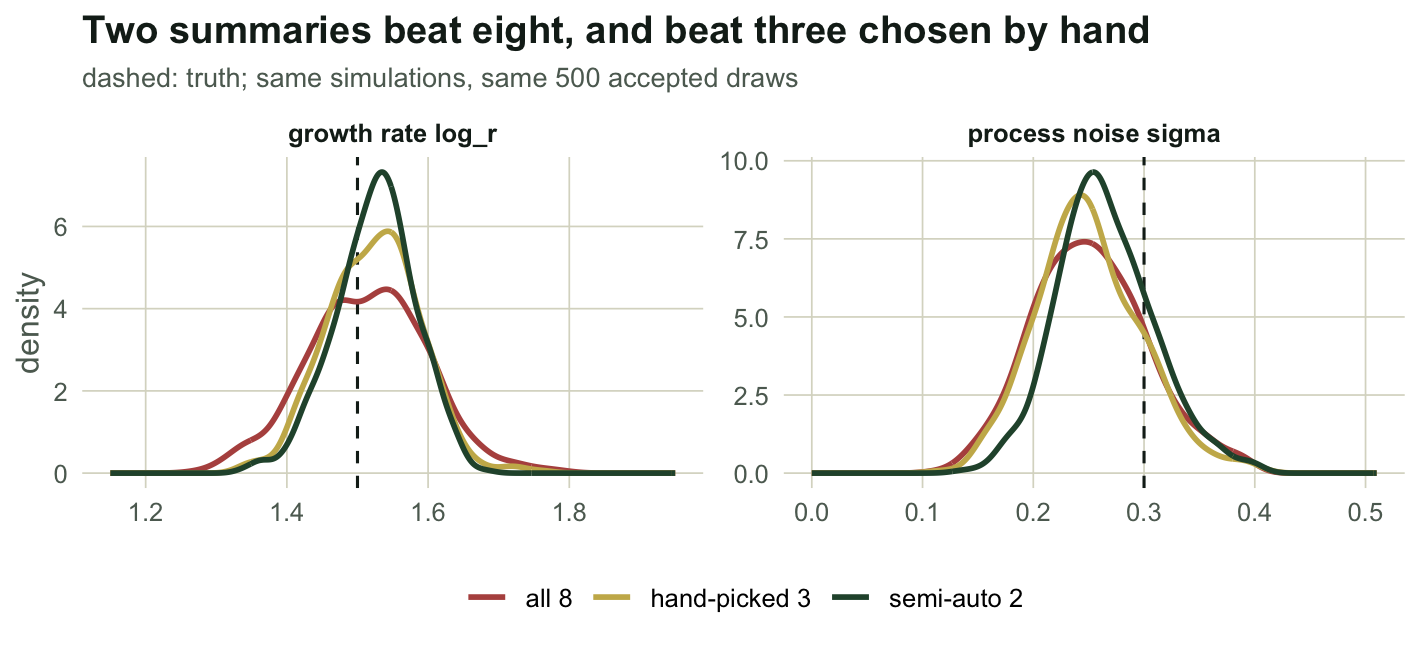

Figure 4: Three ABC posteriors from the same 50,000 simulations and the same 500 accepted draws. The regression compresses eight candidate summaries into one per parameter and beats both the full set and the set an ecologist would pick by hand.

The two projected summaries give a growth-rate posterior with a standard deviation of 0.057 against 0.085 for the full candidate set, and 0.044 against 0.051 for the process noise. The eight-summary distance is not being punished for having bad summaries. It is being punished for having eight of them, exactly as the noise experiment predicted, and the regression is what reads the useful directions out of them and throws the rest away.

Note what did not happen: nobody had to know that the mean count identifies the equilibrium or that the autocorrelation reads the return rate. The regression found the combination. The ecological knowledge went into building the simulator, which is where it belongs.

Where to go next

The honest limits are worth stating plainly. The projection is a regression, so it inherits every regression’s failure modes: a linear or quadratic basis in the candidates may simply not contain a good approximation to the posterior mean, and you will not be warned. If the candidates jointly miss something, no projection recovers it, because the projection is a function of the candidates and nothing else. And the pilot run is a real cost, roughly doubling the simulation bill.

There is also a boundary this post did not cross. Everything above accepts or rejects, which means the tolerance is doing the smoothing. Beaumont, Zhang and Balding (2002) pointed out that you can instead keep a looser tolerance and regress the accepted parameters back onto their summary error, correcting the accepted sample rather than throwing most of it away. That trick, and the sampling schemes that stop proposing from the prior altogether, are where this cluster goes next.

One more thing to sit with. Everything measured here was measured against a truth we had planted ourselves. On real data there is no truth to check the width against, no exact posterior to overlay, and a summary that quietly loses information looks exactly like a summary that does not. That is the uncomfortable part of ABC, and it is a whole post of its own.

Related tutorials

• Approximate Bayesian computation from scratch
• Metropolis-Hastings from scratch
• Choosing a dissimilarity index
• ABC-MCMC and sequential ABC samplers

References

• Beaumont, Zhang, Balding 2002 Genetics 162(4):2025-2035 (10.1093/genetics/162.4.2025)
• Joyce, Marjoram 2008 Statistical Applications in Genetics and Molecular Biology 7(1) (10.2202/1544-6115.1389)
• Beaumont 2010 Annual Review of Ecology, Evolution, and Systematics 41(1):379-406 (10.1146/annurev-ecolsys-102209-144621)
• Fearnhead, Prangle 2012 Journal of the Royal Statistical Society B 74(3):419-474 (10.1111/j.1467-9868.2011.01010.x)
• Blum, Nunes, Prangle, Sisson 2013 Statistical Science 28(2):189-208 (10.1214/12-STS406)
• Prangle 2017 Bayesian Analysis 12(1):289-309 (10.1214/16-BA1002)