library(ggplot2)
library(patchwork)

te_paper  <- "#f5f4ee"
te_ink    <- "#16241d"
te_body   <- "#2c3a31"
te_forest <- "#275139"
te_rust   <- "#b5534e"
te_gold   <- "#c9b458"
te_line   <- "#dad9ca"

theme_datasheet <- function() {
  theme_minimal(base_size = 12) +
    theme(plot.background  = element_rect(fill = te_paper, colour = NA),
          panel.background = element_rect(fill = te_paper, colour = NA),
          panel.grid.major = element_line(colour = te_line, linewidth = 0.3),
          panel.grid.minor = element_blank(),
          text             = element_text(colour = te_body),
          plot.title       = element_text(colour = te_ink, face = "bold"),
          plot.subtitle    = element_text(colour = te_body),
          axis.text        = element_text(colour = te_body))
}Observation error estimated as zero in a Gompertz fit
R
population dynamics
state-space models
time series
density dependence
simulation
ecology tutorial
A Gompertz state-space fit often puts observation error at zero and keeps the whole bias. In R: how often, what the interval covers, and what repairs it.
A colony of grey herons is counted once a year, from the same bank, by whoever is on duty. Thirty years of nest counts go onto the log scale, and the question is how strongly the colony is regulated. The counts carry error, because nests are missed behind leaves and counted twice from two angles, so the analysis is a Gompertz state-space model: a hidden log abundance with density dependence and process noise, observed through a second layer of counting noise. The fit comes back, the optimiser reports success, and the observation standard deviation is exactly zero.
This site has already fitted that model. The post on the Gompertz state-space model builds the Kalman filter by hand, and its Monte Carlo over four hundred series of fifty years finds that “Accounting for observation error roughly halves the bias, which is the payoff the model is designed for.” That average is two states. In a sizeable share of the series the likelihood is maximised with no observation error at all; there the model is the same likelihood as an exact AR(1) fit, it keeps the whole attenuation it was built to remove, and its interval is the AR(1) interval. The other series recover most of the slope. The site’s own fit does not show which state a series is in, because it estimates the log of the variance and so its observation standard deviation never reaches zero.
None of this is new. Dennis and colleagues reported maximum likelihood estimates of one variance sitting on zero in exactly this model in 2006, and compared maximum likelihood with restricted maximum likelihood on first differences; Knape showed in 2008 that, for some parameter values, density dependence and the two variances are only weakly identified once observation error enters; Auger-Methe and colleagues found in 2016 that even simple linear Gaussian state-space models run into estimation problems. The post on checking a MAR(1) model cites all three and already gives the design answer, that “Two hauls on the same day differ only by observation error, which estimates \(\tau^2\) directly.” This post is a demonstration of those results. What it measures is the share of series that land on the zero, what the slope and its interval do in each state, and how much of the damage replicate counts and restricted likelihood undo.
The split has a close relative here. Random effects with too few levels also finds its rates are an average of two states: in singular fits even the correct test rejects a true null at more than twice the nominal rate, and in positive fits it almost never does. What it finds nearly harmless is deleting the random term once the fit is singular: its figure title reads “Deleting the term barely moves the test”. Here the deletion is the harm. A fit on the boundary has silently deleted the observation error, and what it returns is the attenuated slope the model exists to correct.
Two variances and a wall
The model is the one in the Gompertz post: a hidden log abundance \(X_t\) with \(X_{t+1} = \mu + b\,(X_t - \mu) + \varepsilon_t\), \(\varepsilon_t \sim \mathrm{Normal}(0, \sigma_p^2)\), observed as \(Y_t = X_t + \eta_t\), \(\eta_t \sim \mathrm{Normal}(0, \sigma_o^2)\). The filter below is parametrised on the standard deviations and bounded below at zero, so that a zero is a zero.
b_set  <- 0.70            # density dependence, as in the Gompertz post
sp_set <- 0.15            # process SD on the log scale
mu_set <- log(200)        # equilibrium log abundance
tol_ll <- 1e-6            # log-likelihood tie tolerance for the refit at zero

# Kalman filter negative log-likelihood, stationary start, parameters on the SD scale
ssm_nll <- function(par, y, so2_fix = NULL) {
  mu <- par[1]; b <- par[2]; sp2 <- par[3]^2
  so2 <- if (is.null(so2_fix)) par[4]^2 else so2_fix
  m <- mu; P <- sp2 / (1 - b^2); ll <- 0
  for (i in seq_along(y)) {
    Fv <- P + so2; v <- y[i] - m; K <- P / Fv
    ll <- ll - 0.5 * (log(2 * pi * Fv) + v^2 / Fv)
    m <- mu + b * (m + K * v - mu); P <- b^2 * P * (1 - K) + sp2
  }
  -ll
}

# restricted likelihood (Dennis et al. 2006: the likelihood of the first differences),
# computed as the GLS-profiled Kalman likelihood plus its log determinant correction
reml_nll <- function(par, y, so2_fix = NULL) {
  b <- par[1]; sp2 <- par[2]^2
  so2 <- if (is.null(so2_fix)) par[3]^2 else so2_fix
  P <- sp2 / (1 - b^2); m_y <- 0; m_1 <- 0
  e_y <- e_1 <- f_v <- numeric(length(y))
  for (i in seq_along(y)) {
    Fv <- P + so2; K <- P / Fv
    e_y[i] <- y[i] - m_y; e_1[i] <- 1 - m_1; f_v[i] <- Fv
    m_y <- b * (m_y + K * e_y[i]); m_1 <- b * (m_1 + K * e_1[i])
    P <- b^2 * P * (1 - K) + sp2
  }
  s11 <- sum(e_1^2 / f_v); mu_gls <- sum(e_1 * e_y / f_v) / s11
  0.5 * (sum(log(f_v)) + log(s11) + sum((e_y - mu_gls * e_1)^2 / f_v))
}

fit_one <- function(nll, starts, lower, upper, ...) {
  best <- NULL
  for (st in starts) {
    o <- tryCatch(optim(st, nll, ..., method = "L-BFGS-B", lower = lower, upper = upper),
                  error = function(e) NULL)
    if (!is.null(o) && (is.null(best) || o$value < best$value)) best <- o
  }
  best
}
wald_se <- function(nll, par, j, ...) {
  H <- tryCatch(optimHess(par, nll, ...), error = function(e) NULL)
  V <- if (is.null(H)) NULL else tryCatch(solve(H), error = function(e) NULL)
  if (is.null(V) || !is.finite(V[j, j]) || V[j, j] <= 0) NA else sqrt(V[j, j])
}
The likelihood is an even function of \(\sigma_o\), because only \(\sigma_o^2\) enters it. Setting \(\sigma_o = 0\) makes the Kalman gain one at every step, so the filter simply passes the observations through: the first term is the stationary normal density of \(Y_1\) and every later term is the normal density of \(Y_t\) given \(Y_{t-1}\). That is the exact likelihood of a stationary AR(1) process, and it is algebra, not a finding. The check below compares the filter at zero with that likelihood written out directly.
set.seed(2911)
y_chk <- mu_set + as.numeric(arima.sim(list(ar = b_set), 30, sd = sp_set))
par_chk <- c(5.1, 0.55, 0.18)
ar1_direct <- -(dnorm(y_chk[1], par_chk[1], par_chk[3] / sqrt(1 - par_chk[2]^2), log = TRUE) +
  sum(dnorm(y_chk[-1], par_chk[1] + par_chk[2] * (y_chk[-30] - par_chk[1]), par_chk[3], log = TRUE)))
gap_ar1 <- abs(ssm_nll(par_chk, y_chk, so2_fix = 0) - ar1_direct)
At an arbitrary parameter value the two agree to within floating-point rounding. So any series whose likelihood peaks at \(\sigma_o = 0\) gets the slope of an exact AR(1) fit, by construction.
Two consequences follow before any simulation. The slope on the wall is the exact maximum likelihood AR(1) slope, which is close to the least squares slope of the density dependence test but not the same number. And because the likelihood is even in \(\sigma_o\), its derivative in \(\sigma_o\) is zero at zero and so are the cross derivatives with the other parameters; the Wald standard error of \(b\) from the full four parameter Hessian is then the AR(1) standard error. Both are checked in the simulation.
Each fit below runs the bounded optimiser from two starting points taken from the data and from a grid of four slopes crossed with three shares of the variance given to observation error. The grid is there because the likelihood of this model can have more than one peak, as Dennis and colleagues found, and a fit that stops near zero can miss a higher peak elsewhere. The fit is then repeated with \(\sigma_o\) fixed at zero, and the refit is kept whenever its log-likelihood is at least as high as the best free fit to within \(1 \times 10^{-6}\). That refit is what decides the state, not a threshold on \(\hat\sigma_o\): the likelihood is so flat near zero that a bounded optimiser can stop a little short of the wall, and a log-scale optimiser always does.
# two data-based starts, then a grid over the slope and the observation share of the variance
ml_starts <- function(y) {
  n <- length(y); s <- sd(y)
  b0 <- min(max(cor(y[-1], y[-n]), -0.9), 0.9)
  st <- list(c(mean(y), b0, 0.7 * s, 0.1 * s), c(mean(y), 0.5, 0.3 * s, 0.6 * s))
  for (b_st in c(0.2, 0.5, 0.8, 0.95)) for (f_obs in c(0.2, 0.5, 0.8))
    st[[length(st) + 1]] <- c(mean(y), b_st, sqrt((1 - f_obs) * (1 - b_st^2)) * s, sqrt(f_obs) * s)
  st
}
fit_ml <- function(y) {
  n <- length(y); s <- sd(y)
  b0 <- min(max(cor(y[-1], y[-n]), -0.9), 0.9)
  st <- ml_starts(y)
  lo <- c(-Inf, -0.99, 1e-4, 0); hi <- c(Inf, 0.99, Inf, Inf)
  free_2 <- fit_one(ssm_nll, st[1:2], lo, hi, y = y)           # the two data-based starts only
  free_g <- fit_one(ssm_nll, st[-(1:2)], lo, hi, y = y)        # the grid
  free <- if (is.null(free_g) || free_2$value <= free_g$value) free_2 else free_g
  zero <- fit_one(ssm_nll, list(c(mean(y), b0, 0.7 * s), free$par[1:3]), lo[1:3], hi[1:3],
                  y = y, so2_fix = 0)
  wall <- zero$value <= free$value + tol_ll
  list(free = free, zero = zero, wall = wall, wall_2 = zero$value <= free_2$value + tol_ll,
       b = if (wall) zero$par[2] else free$par[2],
       se = if (wall) wald_se(ssm_nll, zero$par, 2, y = y, so2_fix = 0)
            else wald_se(ssm_nll, free$par, 2, y = y))
}
fit_reml <- function(y) {
  n <- length(y); s <- sd(y)
  b0 <- min(max(cor(y[-1], y[-n]), -0.9), 0.9)
  free <- fit_one(reml_nll, list(c(b0, 0.7 * s, 0.1 * s), c(0.5, 0.3 * s, 0.6 * s)),
                  c(-0.99, 1e-4, 0), c(0.99, Inf, Inf), y = y)
  zero <- fit_one(reml_nll, list(c(b0, 0.7 * s)), c(-0.99, 1e-4), c(0.99, Inf), y = y, so2_fix = 0)
  wall <- zero$value <= free$value + tol_ll
  list(wall = wall, b = if (wall) zero$par[1] else free$par[1],
       se = if (wall) wald_se(reml_nll, zero$par, 1, y = y, so2_fix = 0)
            else wald_se(reml_nll, free$par, 1, y = y))
}
The Gompertz post’s own series, split
The first test is on the neighbour’s own simulation. The chunk below copies the Gompertz post’s helper functions unchanged and runs its Monte Carlo chunk line for line, with the same seed, series length and parameters. The only additions keep what that chunk throws away (the fitted observation standard deviation, the log-likelihood and the interval the post builds on the tanh scale) and refit each series with the observation variance fixed at zero. None of the additions draws a random number, so these are the same four hundred series.
# helper functions from the Gompertz state-space post, unchanged
kf_nll <- function(par, y, fixed_so2=NA){
  a<-par[1]; b<-tanh(par[2]); sp2<-exp(par[3])
  so2 <- if(is.na(fixed_so2)) exp(par[4]) else fixed_so2
  n_t<-length(y); xp<-a/(1-b); Pp<-sp2/(1-b^2); ll<-0
  for(t in 1:n_t){
    v<-y[t]-xp; S<-Pp+so2; K<-Pp/S      # innovation, its variance, Kalman gain
    xf<-xp+K*v; Pf<-(1-K)*Pp            # filtered state and variance
    ll<-ll-0.5*(log(2*pi*S)+v*v/S)      # log-likelihood contribution
    xp<-a+b*xf; Pp<-b^2*Pf+sp2          # predict the next state
  }
  -ll
}
fit_gss <- function(y){
  n<-length(y); x0<-y[-n]; x1<-y[-1]; b0<-cov(x0,x1)/var(x0); a0<-mean(x1)-b0*mean(x0)
  vr<-var(x1-(a0+b0*x0)); b0<-min(max(b0,-0.9),0.9)
  st<-c(a0, atanh(b0), log(0.5*vr), log(0.5*vr))
  op<-optim(st, kf_nll, y=y, method="BFGS", hessian=TRUE, control=list(maxit=1000))
  b<-tanh(op$par[2]); V<-tryCatch(solve(op$hessian), error=function(e) matrix(NA,4,4))
  se_tb<-sqrt(V[2,2])
  list(a=op$par[1], b=b, sp=sqrt(exp(op$par[3])), so=sqrt(exp(op$par[4])),
       theta_b=op$par[2], se_tb=se_tb, se_b=(1-b^2)*se_tb, conv=op$convergence, ll=-op$value)
}
naive_b <- function(y){ n<-length(y); cov(y[-n],y[-1])/var(y[-n]) }

# added: the same fit with the observation variance fixed at zero
refit_zero <- function(y){ n<-length(y); x0<-y[-n]; x1<-y[-1]; b0<-cov(x0,x1)/var(x0)
  a0<-mean(x1)-b0*mean(x0); vr<-var(x1-(a0+b0*x0)); b0<-min(max(b0,-0.9),0.9)
  -optim(c(a0, atanh(b0), log(vr)), kf_nll, y=y, fixed_so2=0, method="BFGS",
         control=list(maxit=1000))$value }

# the post's chunk "mc", line for line, plus the stored extras
b_true<-0.70; sp_true<-0.15; so_true<-0.15
Xstar<-log(200); a_true<-(1-b_true)*Xstar; Tlen<-50
nb_so <- nb_ll <- nb_ll0 <- nb_cov <- numeric(400); nb_y <- vector("list", 400)
set.seed(7100); M<-400; nbv<-numeric(M); gbv<-numeric(M); cv<-integer(M)
for(i in 1:M){ x<-numeric(Tlen); x[1]<-Xstar
  for(t in 1:(Tlen-1)) x[t+1]<-a_true+b_true*x[t]+rnorm(1,0,sp_true)
  y<-x+rnorm(Tlen,0,so_true); nbv[i]<-naive_b(y); ff<-fit_gss(y); gbv[i]<-ff$b; cv[i]<-ff$conv
  nb_so[i] <- ff$so; nb_ll[i] <- ff$ll; nb_ll0[i] <- refit_zero(y); nb_y[[i]] <- y
  ci_i <- tanh(ff$theta_b + c(-1, 1) * 1.96 * ff$se_tb)
  nb_cov[i] <- ci_i[1] < b_true & b_true < ci_i[2] }

nb_wall <- nb_ll0 >= nb_ll - tol_ll
nb_ok <- cv == 0
nb_share <- mean(nb_wall[nb_ok])
nb_n_wall <- sum(nb_wall & nb_ok); nb_n_int <- sum(!nb_wall & nb_ok)
nb_b_wall <- mean(gbv[nb_wall & nb_ok]); nb_b_int <- mean(gbv[!nb_wall & nb_ok])
nb_naive_wall <- mean(nbv[nb_wall & nb_ok])
nb_na <- sum(is.na(nb_cov[nb_ok]))
nb_cov_wall <- mean(nb_cov[nb_wall & nb_ok], na.rm = TRUE)
nb_cov_int <- mean(nb_cov[!nb_wall & nb_ok], na.rm = TRUE)
nb_cov_all <- mean(nb_cov[nb_ok], na.rm = TRUE)
# added: the bounded fit of this post, from all its starting points, on the same series
nb_bd <- t(sapply(nb_y, function(y) { m <- fit_ml(y)
  c(ll = -m$free$value, wall = m$wall, b = m$free$par[2]) }))
nb_bw <- nb_bd[, "wall"] == 1
nb_misc <- nb_wall & nb_ok & !nb_bw                   # a higher peak away from zero exists
misc_gain <- nb_bd[, "ll"] - nb_ll0
misc_big <- nb_misc & misc_gain > 0.1
n_misc <- sum(nb_misc); n_misc_big <- sum(misc_big)
n_other_way <- sum(!nb_wall & nb_ok & nb_bw)
bw_share <- mean(nb_bw[nb_ok])
bw_b_wall <- mean(gbv[nb_bw & nb_ok]); bw_naive_wall <- mean(nbv[nb_bw & nb_ok])
bw_b_int <- mean(gbv[!nb_bw & nb_ok])
bw_cov_wall <- mean(nb_cov[nb_bw & nb_ok], na.rm = TRUE)
bw_cov_int <- mean(nb_cov[!nb_bw & nb_ok], na.rm = TRUE)
nb_so_min <- min(nb_so); nb_so_wall_max <- max(nb_so[nb_wall & nb_bw])
nb_thr <- c(mean(nb_so < 1e-3), mean(nb_so < 0.01), mean(nb_so < 0.03))
nb_tol <- c(mean(nb_ll0 >= nb_ll), mean(nb_ll0 >= nb_ll - 1e-3))
The rerun reproduces the post: the naive slope averages 0.385, the state-space slope 0.549 with a standard deviation of 0.226, and 400 of the 400 fits report convergence.
Split by the refit, 124 of those series, a share of 0.310, have a likelihood with no observation error at least as high as the best the post’s own fit reached. On them the state-space slope averages 0.373, and the naive regression slope on the same series averages 0.376: the model has removed none of the bias there. The other 276 series average 0.628. The post’s 0.549 is a blend of the two.
The intervals split the same way. The post’s interval for \(b\), built on the tanh scale, contains the true 0.70 in 0.220 of the series on the wall and in 0.989 of the others, 0.751 overall (2 series with a singular Hessian are left out of these rates).
That rule compares the zero refit with the optimum the post’s own fit found, and the likelihood can have a second peak. This post’s bounded fit, run from all its starting points on the same series, finds a higher likelihood away from zero on 7 of the 124 series. On 3 of them the gain is between 0.32 and 0.50 log-likelihood units and the slope at the higher peak is between 0.90 and 0.94, where the post’s fit had reported 0.023, 0.361, 0.115; on the others the gain is below 0.01. The reverse, a series the post’s fit puts off the wall and the bounded fit puts on it, occurs 0 times. Split by the bounded fit, 0.292 of the series are on the wall; there the post’s slope averages 0.382 against a naive 0.386, and its interval covers 0.214; the other series average 0.618 and cover 0.975. The split barely moves.
The fitted observation standard deviation hides all of this. Because the fit works on the log of the variance, \(\hat\sigma_o\) never goes below 0.00125 on these four hundred series, and a series whose likelihood peaks at zero can still return a \(\hat\sigma_o\) as large as 0.130 with a clean convergence code. A threshold on \(\hat\sigma_o\) misclassifies them: below 0.001 finds 0.000 of the series, below 0.01 finds 0.230, and below 0.03 finds 0.282. The tie tolerance matters much less: requiring the refit to be at least as high with no tolerance at all gives 0.310, and allowing it to fall short by 0.001 gives 0.320.
nb_df <- data.frame(b = gbv[nb_ok],
                    state = factor(ifelse(nb_wall[nb_ok], "fit no better than at zero", "fit better with observation error"),
                                   levels = c("fit no better than at zero", "fit better with observation error")))
nb_lines <- data.frame(x = c(b_true, mean(nbv)), what = c("true slope", "naive mean"))
p_nb <- ggplot(nb_df, aes(b, fill = state)) +
  geom_histogram(binwidth = 0.05, boundary = 0, colour = te_paper, linewidth = 0.2) +
  geom_vline(xintercept = b_true, colour = te_ink, linewidth = 0.8) +
  geom_vline(xintercept = mean(nbv), colour = te_ink, linewidth = 0.8, linetype = "dashed") +
  annotate("text", x = b_true, y = Inf, label = " true 0.70", hjust = 0, vjust = 1.5,
           colour = te_ink, size = 3.5) +
  annotate("text", x = mean(nbv), y = Inf, label = "naive mean ", hjust = 1, vjust = 1.5,
           colour = te_ink, size = 3.5) +
  scale_fill_manual(values = c(te_rust, te_forest), name = NULL) +
  labs(x = "state-space estimate of b", y = "series",
       title = "Four hundred Gompertz fits, split by state",
       subtitle = "the Gompertz post's own simulation: fifty years, both SDs 0.15") +
  theme_datasheet() + theme(legend.position = "bottom")
p_nb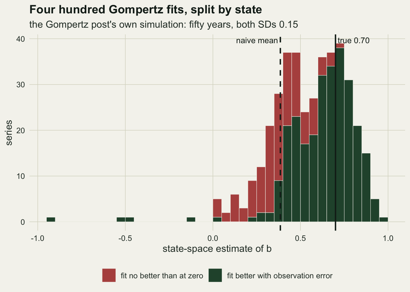
On the wall the fit is an exact AR(1) fit
The neighbour’s chunk has one design. The grid below uses the same process, starts every series from the stationary distribution, and varies the series length (twenty, thirty and fifty years) with the two standard deviations equal, then holds thirty years and halves or doubles the observation standard deviation. Every series also gets a second count in the same year with independent counting error, used only by the repair further down. The replication was fixed before any rate was looked at: four hundred series per length and two hundred per variance ratio cell.
sim_series <- function(t_len, so) {
  x <- numeric(t_len); x[1] <- rnorm(1, mu_set, sp_set / sqrt(1 - b_set^2))
  for (i in 2:t_len) x[i] <- mu_set + b_set * (x[i - 1] - mu_set) + rnorm(1, 0, sp_set)
  list(y1 = x + rnorm(t_len, 0, so), y2 = x + rnorm(t_len, 0, so))
}
one_series <- function(t_len, so) {
  d <- sim_series(t_len, so); y <- d$y1
  ml <- fit_ml(y); rl <- fit_reml(y)
  so2_rep <- mean((d$y1 - d$y2)^2) / 2; y_mean <- (d$y1 + d$y2) / 2; s <- sd(y_mean)
  rep_fit <- fit_one(ssm_nll, list(c(mean(y_mean), 0.5, 0.7 * s)), c(-Inf, -0.99, 1e-4),
                     c(Inf, 0.99, Inf), y = y_mean, so2_fix = so2_rep / 2)
  free_at_zero <- ml$free$par[4] < 1e-3
  se_full <- if (free_at_zero) wald_se(ssm_nll, ml$free$par, 2, y = y) else NA
  r12 <- acf(y, lag.max = 2, plot = FALSE)$acf[2:3]
  c(wall = ml$wall, wall_2 = ml$wall_2, so_free = ml$free$par[4], sp_free = ml$free$par[3], b = ml$b, se = ml$se,
    b_free = ml$free$par[2], b_ar1 = ml$zero$par[2], se_full = se_full,
    b_ols = unname(coef(lm(y[-1] ~ y[-t_len]))[2]), r1 = r12[1], r2 = r12[2],
    b_rep = rep_fit$par[2],
    se_rep = wald_se(ssm_nll, rep_fit$par, 2, y = y_mean, so2_fix = so2_rep / 2),
    reml_wall = rl$wall, b_reml = rl$b, se_reml = rl$se)
}
sim_cell <- function(n_ser, t_len, ratio) {
  out <- as.data.frame(t(replicate(n_ser, one_series(t_len, ratio * sp_set))))
  out$t_len <- t_len; out$ratio <- ratio
  out
}
t_grid <- c(20, 30, 50); ratio_grid <- c(0.5, 2)
n_len <- 400; n_ratio <- 200
set.seed(3290)
cells <- c(lapply(t_grid, function(tl) sim_cell(n_len, tl, 1)),
           lapply(ratio_grid, function(rr) sim_cell(n_ratio, 30, rr)))
names(cells) <- c(sprintf("T%d", t_grid), sprintf("R%.1f", ratio_grid))
covers <- function(b, se) ifelse(is.na(se), NA, abs(b - b_set) < 1.96 * se)
summ <- function(r) {
w <- r$wall == 1; fz <- r$so_free < 1e-3
cv_ml <- covers(r$b, r$se); cv_rep <- covers(r$b_rep, r$se_rep)
cv_reml <- covers(r$b_reml, r$se_reml); rw <- r$reml_wall == 1
c(t_len = r$t_len[1], ratio = r$ratio[1], n = nrow(r), wall = mean(w),
n_wall = sum(w), n_int = sum(!w), free_zero_in_wall = mean(fz[w]),
wall_2 = mean(r$wall_2 == 1), n_moved = sum(r$wall_2 == 1 & !w), n_b_lo = sum(r$b < -0.989),
n_moved_hi = sum(r$wall_2 == 1 & !w & r$b > 0.5), n_moved_neg = sum(r$wall_2 == 1 & !w & r$b < 0),
sp_zero = mean(r$sp_free < 2e-4),
b_all = median(r$b), b_wall = median(r$b[w]), b_int = median(r$b[!w]),
ar1_wall = median(r$b_ar1[w]), ols_wall = median(r$b_ols[w]),
gap_ar1 = max(abs(r$b_free - r$b_ar1)[fz]), gap_ols = max(abs(r$b - r$b_ols)[w]),
gap_se = max(abs(r$se_full - r$se)[fz & w], na.rm = TRUE),
n_na = sum(is.na(cv_ml)), se_wall = median(r$se[w], na.rm = TRUE),
cov_all = mean(cv_ml, na.rm = TRUE), cov_wall = mean(cv_ml[w], na.rm = TRUE),
cov_int = mean(cv_ml[!w], na.rm = TRUE),
screen = mean((r$r2 <= r$r1^2) == w),
screen_pass = mean(r$r2 <= r$r1^2), screen_ppv = mean(w[r$r2 <= r$r1^2]),
screen_npv = mean(!w[r$r2 > r$r1^2]),
b_rep = median(r$b_rep), n_na_rep = sum(is.na(cv_rep)),
cov_rep = mean(cv_rep, na.rm = TRUE),
cov_rep_wall = mean(cv_rep[w], na.rm = TRUE), cov_rep_int = mean(cv_rep[!w], na.rm = TRUE),
reml_wall = mean(rw), b_reml = median(r$b_reml), n_na_reml = sum(is.na(cv_reml)),
reml_pin = mean(r$b_reml > 0.989), n_reml_pin_na = sum(is.na(cv_reml[r$b_reml > 0.989])),
b_reml_nopin = median(r$b_reml[r$b_reml <= 0.989]),
cov_reml_miss = mean(ifelse(is.na(cv_reml), FALSE, cv_reml)),
cov_reml = mean(cv_reml, na.rm = TRUE),
cov_reml_wall = mean(cv_reml[rw], na.rm = TRUE), cov_reml_int = mean(cv_reml[!rw], na.rm = TRUE),
reml_in_ml = mean(w[rw]))
}
tab <- as.data.frame(t(sapply(cells, summ)))
g <- function(cell, what) tab[cell, what]
mcse <- function(p, n) sqrt(p * (1 - p) / n)At thirty years with equal standard deviations, 0.360 of the series have a likelihood on the wall at least as high as the best free fit from all the starting points, 144 of 400. The bounded optimiser on its own had already put \(\hat\sigma_o\) below 0.001 in 0.979 of those; the refit caught the rest. The two data-based starts alone would have put 0.372 there: on 5 series the grid found a higher peak away from zero, 2 of them with a slope above 0.5 and 3 with a negative one. In 2 thirty-year series (13 over all cells) the best free fit puts the slope on its lower bound of -0.99; they count as off the wall. The process standard deviation never sat at its lower limit in any cell (share 0.000 at most): the wall this model hits is the observation error’s.
The algebra checks out on the series where the free fit itself reached zero. Its slope differs from the separately fitted exact AR(1) slope by at most \(1.3 \times 10^{-5}\), and its standard error from the full four parameter Hessian differs from the AR(1) standard error by at most \(3.6 \times 10^{-6}\). The least squares slope is a different estimator: its median on the wall series is 0.379 against 0.382 for the exact fit, close on average, but single series differ by up to 0.116.
The medians carry the two states. The state-space slope has a median of 0.539 over all series, 0.382 on the wall and 0.688 off it, against a true 0.70.
c30 <- cells[["T30"]]
c30$state <- factor(ifelse(c30$wall == 1, "likelihood peaks at zero", "positive observation error"),
                    levels = c("likelihood peaks at zero", "positive observation error"))
p_ar1 <- ggplot(c30, aes(b_ar1, b_free, colour = state)) +
  geom_abline(slope = 1, intercept = 0, colour = te_body, linetype = "dashed", linewidth = 0.4) +
  geom_point(size = 1.4, alpha = 0.75) +
  scale_colour_manual(values = c(te_rust, te_forest), name = NULL) +
  coord_equal(xlim = c(-1, 1), ylim = c(-1, 1)) +
  labs(x = "exact AR(1) slope", y = "state-space slope, free fit",
       title = "Free fit against exact AR(1)") +
  guides(colour = guide_legend(nrow = 2, override.aes = list(size = 2.5))) +
  theme_datasheet() + theme(legend.position = "bottom")
p_ols <- ggplot(c30[c30$wall == 1, ], aes(b_ols, b_ar1)) +
  geom_abline(slope = 1, intercept = 0, colour = te_body, linetype = "dashed", linewidth = 0.4) +
  geom_point(size = 1.4, alpha = 0.75, colour = te_rust) +
  coord_equal(xlim = c(-1, 1), ylim = c(-1, 1)) +
  labs(x = "least squares AR(1) slope", y = "exact AR(1) slope",
       title = "Wall series only") +
  theme_datasheet()
p_ar1 + p_ols + plot_annotation(theme = theme_datasheet())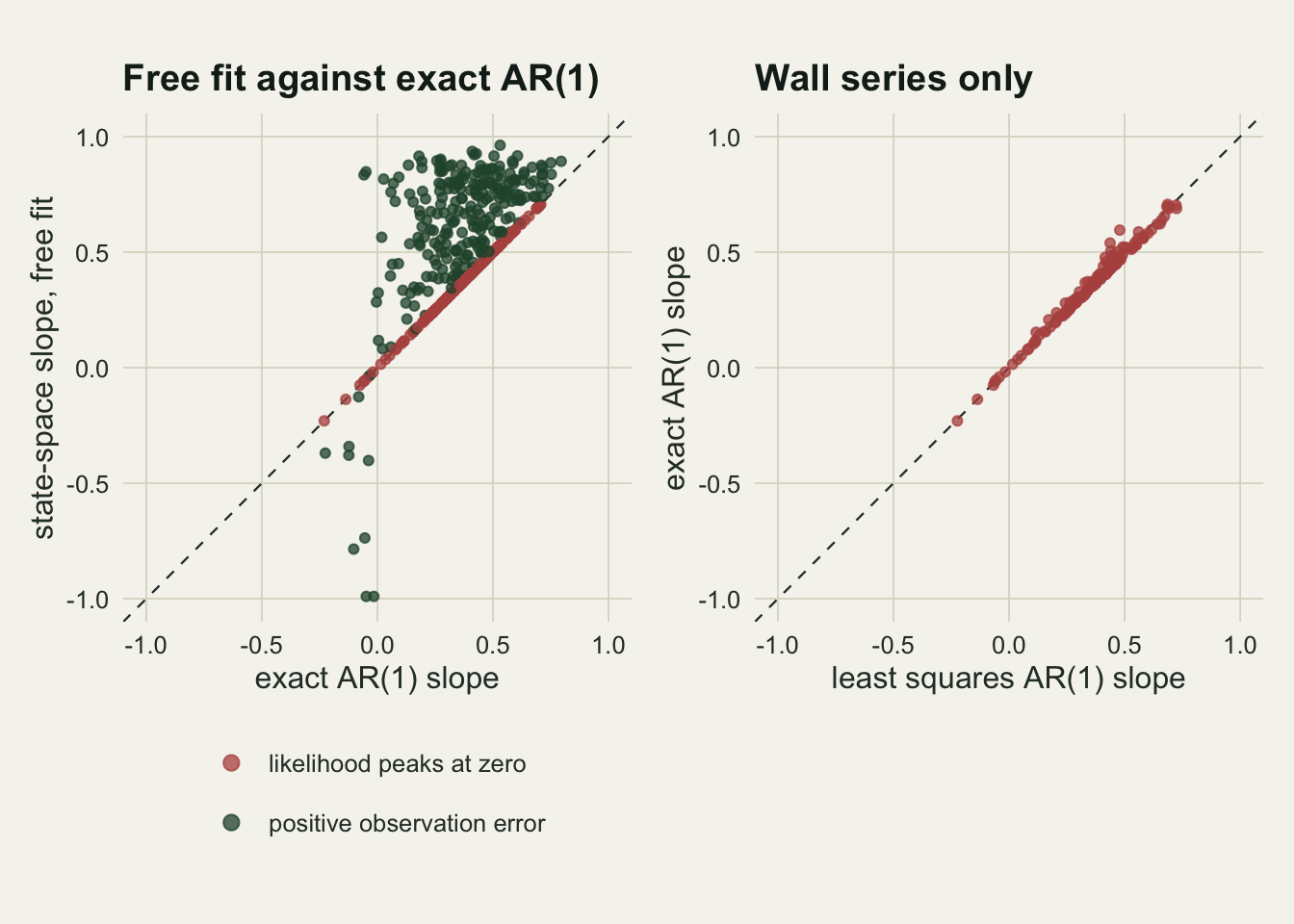
Coverage in the two states
The state is visible to the analyst: a fit that lands on the wall says so, once the refit is run. So the useful coverage is the conditional one. The rates below count a series as covered when its Wald interval, estimate plus or minus 1.96 standard errors, contains the true slope; series with a singular Hessian are counted and left out.
cov_long <- do.call(rbind, lapply(rownames(tab), function(k) {
  n_w <- tab[k, "n_wall"]; n_i <- tab[k, "n_int"]; n_a <- tab[k, "n"]
  data.frame(cell = k, t_len = tab[k, "t_len"], ratio = tab[k, "ratio"],
             arm = c("ML, likelihood peaks at zero", "ML, positive observation error",
                     "ML, all series", "two counts a year"),
             cover = c(tab[k, "cov_wall"], tab[k, "cov_int"], tab[k, "cov_all"], tab[k, "cov_rep"]),
             n = c(n_w, n_i, n_a, n_a))
}))
cov_long$se <- mcse(cov_long$cover, cov_long$n)
cov_long$arm <- factor(cov_long$arm, levels = unique(cov_long$arm))
gap_30 <- g("T30", "cov_int") - g("T30", "cov_wall")
na_total <- sum(tab$n_na); na_rep <- sum(tab$n_na_rep); na_reml <- sum(tab$n_na_reml)
At thirty years the interval covers 0.542 of the time on the wall (Monte Carlo standard error 0.042) and 0.965 off it (0.012), a gap of 0.423; over all series it covers 0.812. At twenty years the wall takes 0.450 of the series and the two coverages are 0.611 and 0.904. At fifty years the wall share falls to 0.265, but the series that still land there are worse off, covering 0.264. Their median slope, 0.374, is no closer to the truth than at thirty years (0.382), while the AR(1) interval narrows as the series lengthens (median standard error on the wall 0.170 at thirty years, 0.131 at fifty), so the same bias is reported with more confidence; the interior covers 0.959. Across all cells 5 maximum likelihood fits had a singular Hessian, as did 7 repaired fits and 52 REML fits; all are counted and left out of their rates.
The variance ratio decides how much the wall costs. With the observation standard deviation at half the process one, 0.460 of the series land on the wall, more than with equal variances, but the attenuation is smaller and their slope has a median of 0.514, so the interval covers 0.761: better than at equal variances, still well short of nominal. With the observation standard deviation at twice the process one, 0.460 land on the wall, their median slope is 0.143, and the interval covers 0.130 of the time there and 0.895 elsewhere.
arm_cols <- c(te_rust, te_forest, te_body, te_gold)
p_t <- ggplot(cov_long[cov_long$ratio == 1, ], aes(t_len, cover, colour = arm)) +
  geom_hline(yintercept = 0.95, colour = te_body, linetype = "dashed", linewidth = 0.4) +
  geom_errorbar(aes(ymin = cover - 2 * se, ymax = cover + 2 * se), width = 1.2, linewidth = 0.4) +
  geom_line(linewidth = 0.9) + geom_point(size = 2.2) +
  scale_colour_manual(values = arm_cols, name = NULL) +
  scale_x_continuous(breaks = t_grid) + scale_y_continuous(limits = c(0, 1)) +
  labs(x = "years in the series", y = "coverage of the true slope",
       title = "Equal standard deviations", subtitle = "dashed: nominal 0.95") +
  theme_datasheet() + theme(legend.position = "none")
p_r <- ggplot(cov_long[cov_long$t_len == 30, ], aes(ratio, cover, colour = arm)) +
  geom_hline(yintercept = 0.95, colour = te_body, linetype = "dashed", linewidth = 0.4) +
  geom_errorbar(aes(ymin = cover - 2 * se, ymax = cover + 2 * se), width = 0.06, linewidth = 0.4) +
  geom_line(linewidth = 0.9) + geom_point(size = 2.2) +
  scale_colour_manual(values = arm_cols, name = NULL) +
  scale_x_log10(breaks = c(0.5, 1, 2)) + scale_y_continuous(limits = c(0, 1)) +
  guides(colour = guide_legend(nrow = 2)) +
  labs(x = "observation SD / process SD", y = NULL,
       title = "Thirty years", subtitle = "bars: two Monte Carlo SEs") +
  theme_datasheet() + theme(legend.position = "bottom")
p_t + p_r + plot_layout(guides = "collect") +
  plot_annotation(theme = theme_datasheet() + theme(legend.position = "bottom"))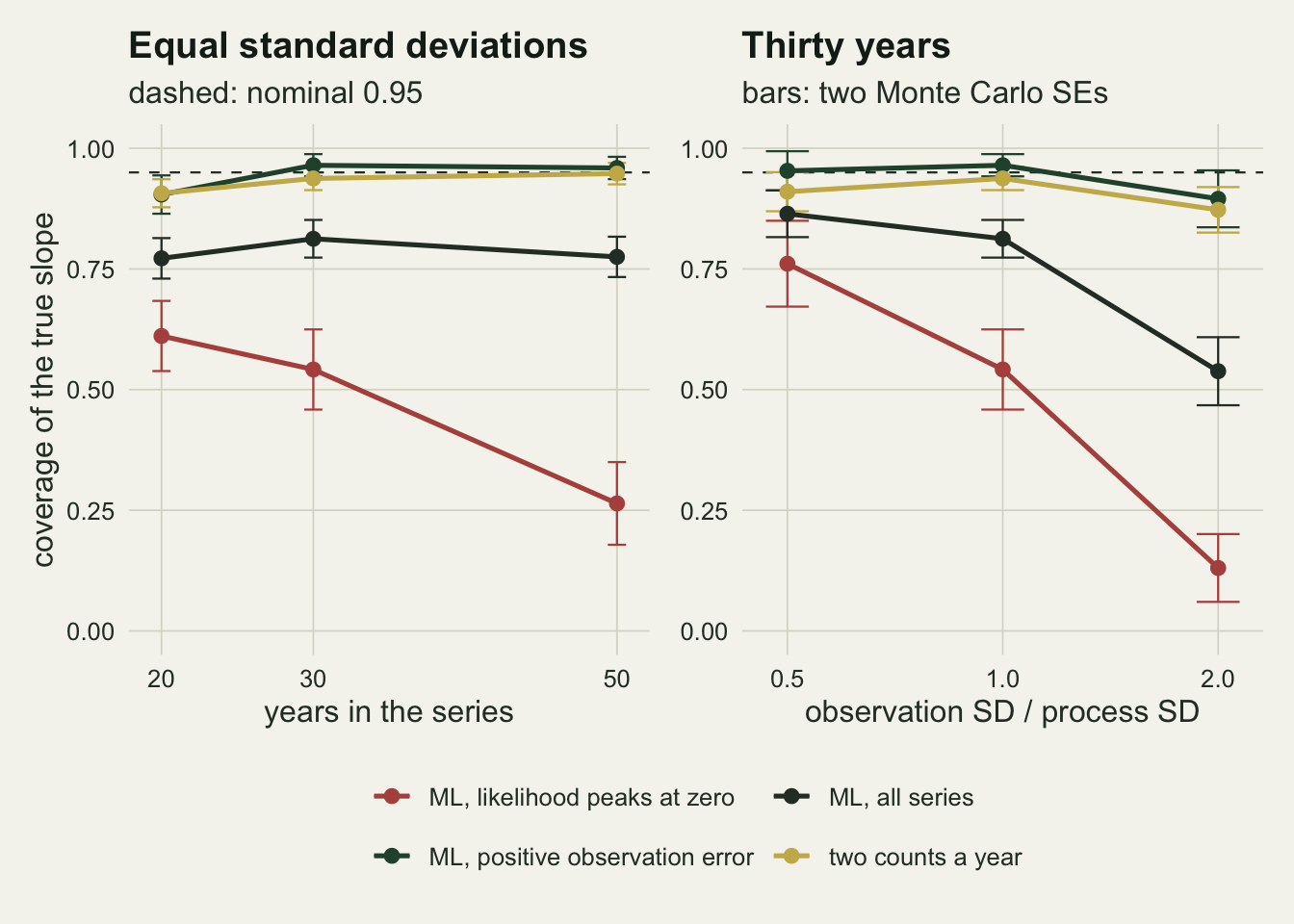
Which series land on the wall
Whether a series ends on the wall is close to a question about its first two sample autocorrelations. A stationary AR(1) process has a lag-two autocorrelation equal to the square of its lag-one autocorrelation. Independent observation error multiplies every autocorrelation beyond lag zero by the same factor, the share of the variance that is signal, so the square of the lag-one value shrinks by that factor twice and the lag-two value only once: in the population, the lag-two value ends up above the square of the lag-one value. A series whose sample autocorrelations show \(r_2 \le r_1^2\) looks like a clean AR(1) process, and the likelihood has no reason to add observation error.
parab <- data.frame(r1 = seq(-0.4, 1, by = 0.01)); parab$r2 <- parab$r1^2
ggplot(c30, aes(r1, r2, colour = state)) +
  geom_line(data = parab, aes(r1, r2), inherit.aes = FALSE, colour = te_ink, linewidth = 0.7) +
  geom_point(size = 1.5, alpha = 0.75) +
  scale_colour_manual(values = c(te_rust, te_forest), name = NULL) +
  annotate("text", x = 0.95, y = 0.95^2, label = "r2 = r1 squared ", hjust = 1, vjust = -0.6,
           colour = te_ink, size = 3.5) +
  labs(x = "lag-one sample autocorrelation r1", y = "lag-two sample autocorrelation r2",
       title = "The wall is almost a moment condition",
       subtitle = "thirty-year series, equal standard deviations") +
  theme_datasheet() + theme(legend.position = "bottom")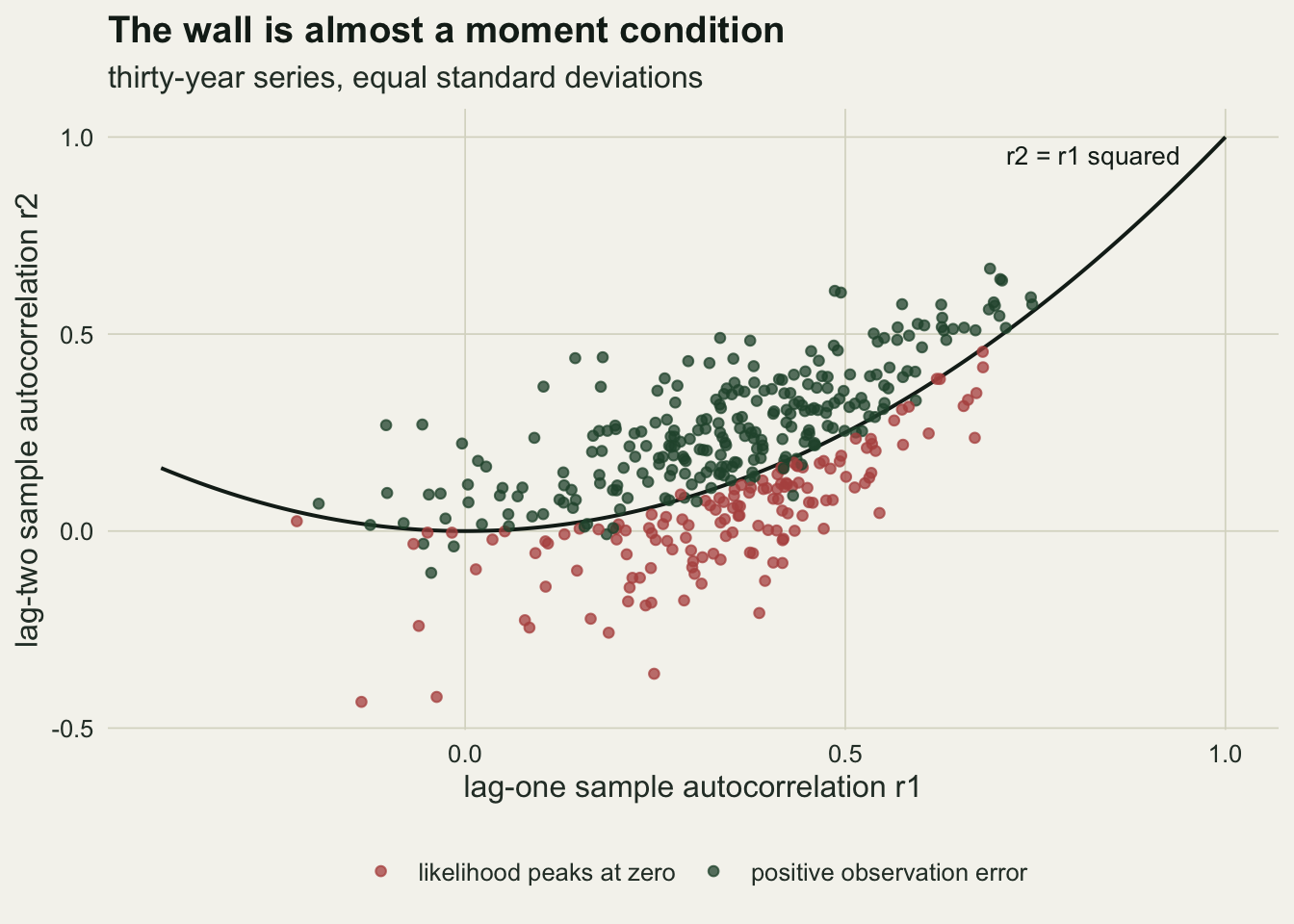
The screen \(r_2 \le r_1^2\) agrees with the refit in 0.945 of the thirty-year series, 0.927 at twenty years and 0.955 at fifty. At thirty years 0.405 of the series show \(r_2 \le r_1^2\), and 0.877 of those end on the wall; of the series that do not show it, 0.992 end off the wall. It is not a separate diagnosis. It is the wall restated in two numbers that can be read off before any model is fitted, and its use is as a warning: a series with \(r_2 \le r_1^2\) is likely to hand back a state-space fit with no observation error, whatever the counting protocol was.
Replicate counts, and restricted likelihood
The repair both neighbours recommend is a design change. Count twice in the same season, with independent error: the difference between the two counts contains no process variation, so half its mean square estimates \(\sigma_o^2\), and the mean of the two counts has observation variance \(\sigma_o^2 / 2\), which is fixed at that estimate while the rest of the model is fitted to the annual means. This uses twice the fieldwork of the single-count arms.
At thirty years with equal variances the repaired interval covers 0.938 (0.944 on the series whose single-count fit was on the wall, 0.934 on the rest), 0.907 at twenty years and 0.948 at fifty. What it does not restore is the point estimate: the median repaired slope is 0.602 at thirty years and 0.624 at fifty, still short of 0.70. The Monte Carlo standard error of the thirty-year coverage is 0.012. With the observation standard deviation at twice the process one the repair covers 0.872.
Restricted maximum likelihood is the analysis-side answer Dennis and colleagues compare with maximum likelihood. It maximises the likelihood of the first differences of the log counts, which does not contain the mean; the version in the code computes it through the Kalman filter as the likelihood profiled over the mean plus a log determinant correction, a standard identity for restricted likelihood. The chunk below checks it against the likelihood of the differences written out as a multivariate normal, then summarises the REML fits, which were run on the same single-count series with the same refit at zero.
reml_diff <- function(par, y) {
  b <- par[1]; sp2 <- par[2]^2; so2 <- par[3]^2
  w <- diff(y); n <- length(w); h <- 0:(n + 1)
  gy <- sp2 * b^h / (1 - b^2); gy[1] <- gy[1] + so2
  gw <- 2 * gy[1:n] - gy[2:(n + 1)] - c(gy[2], gy[1:(n - 1)])
  R <- chol(toeplitz(gw)); z <- backsolve(R, w, transpose = TRUE)
  sum(log(diag(R))) + 0.5 * sum(z^2)
}
par_try <- list(c(0.7, 0.15, 0.15), c(0.3, 0.1, 0.02), c(0.9, 0.2, 0), c(-0.2, 0.05, 0.3))
gap_reml <- max(abs(sapply(par_try, function(p) reml_nll(p, y_chk) - reml_diff(p, y_chk))))
reml_tab <- tab[, c("t_len", "ratio", "wall", "reml_wall", "b_reml", "cov_reml",
                    "cov_reml_wall", "cov_reml_int", "reml_in_ml")]
Across four arbitrary parameter values the two versions agree to within floating-point rounding. At thirty years REML puts 0.297 of the series on the wall against 0.360 for maximum likelihood, and 0.966 of its wall series are also on the maximum likelihood wall. Its median slope is 0.654, against 0.539 for maximum likelihood, but part of that comes from a second wall: REML puts the slope on its upper bound of 0.99 in 0.102 of the thirty-year series (0.128 at twenty years), and without them its median is 0.613. Its interval covers 0.852 overall, 0.723 on its own wall and 0.910 off it. Those rates leave out the 14 thirty-year series with a singular Hessian, 13 of them with the slope on the upper bound; counted as misses, the overall coverage is 0.823, against 0.812 for maximum likelihood with none left out. At fifty years the figures are 0.203 on the wall and 0.820 coverage (0.807 with the singular fits as misses). So restricted likelihood shrinks the wall without removing it, and adds a second one at the upper bound of the slope. On these runs its median is closer to the truth, with or without the series on that bound, and once the singular fits are counted its overall coverage is about the same as maximum likelihood’s at thirty years and a little higher at fifty, but on its own wall the interval still misses far more often than the nominal rate allows. Of the arms tried here, only the replicate counts, which bring information the single series does not contain, bring the coverage close to nominal.
What to report
Report whether the observation variance came out at zero, and say how that was established. With a log-variance fit the printed \(\hat\sigma_o\) cannot be zero, so refit with the observation variance fixed at zero and compare the two log-likelihoods; if the refit is at least as high, the fit is on the wall and should be described as an AR(1) fit to the counts. Fit from several starting points first, because the likelihood can have a second peak away from zero; then the refit at zero is one extra call to optim.
If the fit is on the wall, do not report its slope as corrected for observation error. It is the exact AR(1) slope with the AR(1) interval, and in these simulations that interval covered the truth in 0.542 of the wall series at thirty years and 0.264 at fifty. The honest statement is that the series alone could not separate counting error from process noise, and that the density dependence estimate carries whatever attenuation the counting error causes.
Report \(r_1\) and \(r_2\) alongside the fit. They take one line to compute, and a reader who sees \(r_2 \le r_1^2\) knows, before it runs, that the state-space fit will usually come back with no observation error.
If the counts can be repeated within the season, do it and fix the observation variance from the replicates, as both neighbouring posts advise. Here every year was counted twice; replicates in only some years were not simulated. The repair restored the interval but not the point estimate, so report the repaired interval and not only the repaired slope.
When summarising a simulation study of a model like this, split the results by state. An average over series that sit on the wall and series that do not describes neither kind of series.
Honest limits
The observation layer here is Gaussian on the log scale. Real counts are often Poisson or negative binomial, and a Poisson layer has no Kalman filter; the post on particle MCMC for state space models fits one. Whether a similar share of series lands on a wall under a count observation model was not measured.
Only one process was simulated: \(b = 0.70\), a process standard deviation of 0.15, and three observation to process ratios. The wall share moved with the variance ratio, and not monotonically; how it moves with the strength of density dependence was not measured, so none of the rates above should be carried to a much weaker or much stronger regulation without rerunning the code.
The generator starts every series from its stationary distribution, which matches the stationary start of the filter. The Gompertz post’s own series start at the equilibrium, which is a slight mismatch, and the split held there too, but a series that starts far from equilibrium (a reintroduction, a recovery after a crash) is outside what either simulation covers.
The intervals are Wald intervals from the Hessian, as in the Gompertz post. Profile likelihood or bootstrap intervals may behave differently on the wall and were not tried. The repair fixes the observation variance at its replicate estimate and ignores the uncertainty in that estimate, which matters more the fewer years of paired counts there are; that was not measured.
The repair assumes the two counts in a year have independent errors of the same size. Two observers on the same morning from the same bank may share much of their error (the same nests hidden by the same leaves), in which case the difference underestimates the observation variance and the repair is partial. Replicates are worth most when they are independent by design, such as different vantage points or different days within the season.
The restricted likelihood arm is one implementation, with the same bounds and refit rule as the maximum likelihood arm but only its two data-based starting points, so a second peak of the restricted likelihood was not searched for. The repaired fit, with the observation variance fixed, was run from a single starting point, so the same holds for it. The REML arm answers whether restricted likelihood changes the picture on these series, not how the estimator behaves in general.
References
Dennis B, Ponciano JM, Lele SR, Taper ML, Staples DF 2006 Ecological Monographs 76(3):323-341 (10.1890/0012-9615(2006)76[323:EDDPNA]2.0.CO;2)
Knape J 2008 Ecology 89(11):2994-3000 (10.1890/08-0071.1)
Auger-Methe M, Field C, Albertsen CM, Derocher AE, Lewis MA, Jonsen ID, Mills Flemming J 2016 Scientific Reports 6:26677 (10.1038/srep26677)