---
title: "Checking a MAR(1) model"
description: "In a simulated community, observation error drags every MAR(1) stability metric towards calm while residual diagnostics stay silent. Here is the size of it."
date: "2026-06-11 11:00"
categories: [R, MAR models, model diagnostics, time series, ecology tutorial]
image: thumbnail.png
image-alt: "Estimated interaction strength and community return rate falling steadily as observation error variance increases."
date-modified: "2026-10-14"
---
*Corrected 14 October 2026: the post said the observation error variance is not in the data, and that observation error always pushes every stability metric the same way; it now says a single short series pins that variance down only weakly, and states the direction for the community simulated here rather than for every community.*
*Corrected 7 October 2026: the checklist said synchronised species have unidentifiable interactions; as the post on interaction strengths now says, such interactions stay identified but are estimated much less precisely, and the checklist now says so.*
*Corrected 1 October 2026: the return rates and determinant indices for each noise level were those of the averaged fitted matrix and are now averages over the individual fits, so the return rate shrinks less than the post said, though it still falls steadily as observation error grows. The post also no longer puts part of the low Ljung-Box rate down to correlated residuals, says the attenuated model fails its residual check no more often than a correct one rather than never, and notes that the counting error it calls modest is larger than the process variance of two of the four species.*
*Corrected 30 September 2026: the post said the residuals are white and that attenuation leaves no serial correlation behind; a state observed with error does leave a small residual autocorrelation, which Ljung-Box has too little power to detect in a short series, and the post now says so.*
The three previous posts built a MAR(1) analysis: [the fit](../fitting-a-mar1-model/), [the interaction coefficients](../interaction-strengths-from-time-series/), [the stability metrics](../stability-from-a-mar1-model/). Every number in that chain comes out of one matrix, $B$, and inherits whatever is wrong with it.
This post is about the largest thing that is wrong with it. It has three properties that make it worse than an ordinary nuisance: it is big, in the community simulated here it pushes every stability metric the same way, and the standard diagnostics do not see it.
```{r}
#| label: setup
#| code-fold: true
#| code-summary: "Setup: packages, colours and plot theme"
#| results: hide
#| message: false
#| warning: false
#| fig-show: hide
library(ggplot2)
library(grid)

te_ink    <- "#16241d"
te_forest <- "#275139"
te_gold   <- "#c9b458"
te_rust   <- "#b5534e"
te_sage   <- "#93a87f"
te_line   <- "#dad9ca"
te_muted  <- "#5d6b61"

theme_te <- function(base_size = 12) {
  theme_minimal(base_size = base_size) +
    theme(
      text             = element_text(colour = te_ink),
      plot.title       = element_text(face = "bold", size = rel(1.02), colour = te_ink),
      plot.subtitle    = element_text(colour = te_muted, size = rel(0.88)),
      axis.title       = element_text(colour = te_ink, size = rel(0.92)),
      axis.text        = element_text(colour = te_muted, size = rel(0.82)),
      panel.grid.major = element_line(colour = te_line, linewidth = 0.3),
      panel.grid.minor = element_blank(),
      panel.background = element_rect(fill = "#f5f4ee", colour = NA),
      plot.background  = element_rect(fill = "#f5f4ee", colour = NA),
      legend.position  = "bottom",
      legend.title     = element_text(size = rel(0.82)),
      legend.text      = element_text(size = rel(0.78)),
      legend.key.size  = unit(0.8, "lines")
    )
}

two_panel <- function(p1, p2) {
  grid.newpage()
  pushViewport(viewport(layout = grid.layout(1, 2)))
  print(p1, vp = viewport(layout.pos.row = 1, layout.pos.col = 1))
  print(p2, vp = viewport(layout.pos.row = 1, layout.pos.col = 2))
}

Btrue <- matrix(c( 0.50, -0.10, -0.35,  0.00,
                  -0.15,  0.60,  0.00,  0.00,
                   0.30,  0.00,  0.45, -0.30,
                   0.00,  0.00,  0.25,  0.55), 4, 4, byrow = TRUE)
Atrue <- c(1.20, 0.90, 0.40, 0.30)
Strue <- matrix(c(0.09, 0.03, 0, 0, 0.03, 0.09, 0, 0,
                  0, 0, 0.04, 0.01, 0, 0, 0.01, 0.04), 4, 4, byrow = TRUE)
p <- 4

sim_mar1 <- function(n, A, B, S, seed, burn = 200) {
  set.seed(seed); p <- length(A); L <- chol(S)
  x <- solve(diag(p) - B, A); X <- matrix(0, n, p)
  for (t in seq_len(burn + n)) {
    x <- A + B %*% x + as.vector(rnorm(p) %*% L)
    if (t > burn) X[t - burn, ] <- x
  }
  X
}
mar1_cls <- function(X) {
  n <- nrow(X); Y <- X[-1, , drop = FALSE]; D <- cbind(1, X[-n, , drop = FALSE])
  cf <- solve(crossprod(D), crossprod(D, Y)); E <- Y - D %*% cf
  list(A = cf[1, ], B = t(cf[-1, , drop = FALSE]), Sigma = crossprod(E) / nrow(Y), E = E)
}
```
## The problem: you never count the community, you sample it
MAR(1) treats $X_t$ as the community's log abundance. What you have is a net haul, a quadrat, a transect. The count carries sampling error on top of the real state, and that error is not part of the model as written. Write $\tau^2$ for its variance.
Add it to the simulation and refit, three hundred times per noise level.
```{r}
#| label: attenuation
tau_grid <- c(0, 0.02, 0.05, 0.10, 0.20)

att <- do.call(rbind, lapply(tau_grid, function(tau2) {
  Bh <- array(0, c(300, p, p)); rr <- dt <- numeric(300)
  for (m in 1:300) {
    Xm <- sim_mar1(60, Atrue, Btrue, Strue, seed = 7000 + m)
    set.seed(107000 + m)
    B <- mar1_cls(Xm + matrix(rnorm(60 * p, 0, sqrt(tau2)), 60, p))$B
    Bh[m, , ] <- B
    rr[m] <- max(Mod(eigen(B)$values))
    dt[m] <- abs(det(B))^(2 / p)
  }
  Bm <- apply(Bh, c(2, 3), mean)
  data.frame(tau2 = tau2,
             mean_diag = mean(diag(Bm)),
             pct_of_truth = 100 * mean(diag(Bm)) / mean(diag(Btrue)),
             return_rate = mean(rr),
             det_index = mean(dt))
}))
round(att, 4)
```
Read the table down, not across.
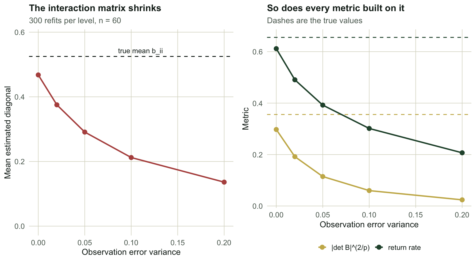
At $\tau^2 = 0$, with perfect observation, the mean diagonal is already `r sprintf("%.0f", att$pct_of_truth[1])` per cent of the truth. That is the small-sample bias from the [previous post](../interaction-strengths-from-time-series/), and on its own it is a mild annoyance.
At $\tau^2 = `r sprintf("%.2f", att$tau2[3])`$, which is a modest amount of counting error next to the process variance of `r sprintf("%.2f", Strue[1,1])` in the first two species but more than the `r sprintf("%.2f", Strue[3,3])` of the other two, the diagonal is down to `r sprintf("%.0f", att$pct_of_truth[3])` per cent. At $\tau^2 = `r sprintf("%.2f", att$tau2[5])`$ it is `r sprintf("%.0f", att$pct_of_truth[5])` per cent. The interaction matrix has lost three quarters of itself.
Now look at what that does to the stability metrics, which is the part that matters. The true return rate is `r sprintf("%.4f", max(Mod(eigen(Btrue)$values)))`. Computed fit by fit and averaged at each noise level, the estimates run `r paste(sprintf("%.4f", att$return_rate), collapse = ", ")` as the observation error grows.
> **The community looks more stable the worse your data is.** Sloppier counting buys you a faster return rate, a lower determinant index, and a more comfortable story about resilience.
That is not a random error you can average away across studies. It is a systematic gradient, and it runs in the direction of the answer people like.
```{r}
#| label: fig-attenuation
#| fig-width: 8
#| fig-height: 4.4
#| fig-cap: "Left: the mean estimated diagonal against observation error variance, with the truth marked. Right: the two headline stability metrics falling with the same noise. Every point is 300 refits of the identical community."
#| fig-alt: "Two panels. Left, a line falling steeply from just under the true mean diagonal towards zero as observation error grows. Right, two lines for return rate and the determinant index both falling steeply away from their true values."
p1 <- ggplot(att, aes(tau2, mean_diag)) +
  geom_hline(yintercept = mean(diag(Btrue)), colour = te_ink, linetype = 2, linewidth = 0.5) +
  annotate("text", x = 0.11, y = mean(diag(Btrue)) + 0.018, label = "true mean b_ii",
           colour = te_ink, size = 3) +
  geom_line(colour = te_rust, linewidth = 0.8) +
  geom_point(colour = te_rust, size = 2.2) +
  ylim(0, 0.58) +
  labs(title = "The interaction matrix shrinks",
       subtitle = "300 refits per level, n = 60",
       x = "Observation error variance", y = "Mean estimated diagonal") +
  theme_te(11)

met <- rbind(data.frame(tau2 = att$tau2, v = att$return_rate, w = "return rate",
                        truth = max(Mod(eigen(Btrue)$values))),
             data.frame(tau2 = att$tau2, v = att$det_index, w = "|det B|^(2/p)",
                        truth = abs(det(Btrue))^(2 / p)))

p2 <- ggplot(met, aes(tau2, v, colour = w)) +
  geom_hline(aes(yintercept = truth, colour = w), linetype = 2, linewidth = 0.5) +
  geom_line(linewidth = 0.8) +
  geom_point(size = 2.2) +
  scale_colour_manual(values = c(`return rate` = te_forest, `|det B|^(2/p)` = te_gold)) +
  labs(title = "So does every metric built on it",
       subtitle = "Dashes are the true values",
       x = "Observation error variance", y = "Metric", colour = NULL) +
  theme_te(11)

two_panel(p1, p2)
```
## The diagnostics are silent
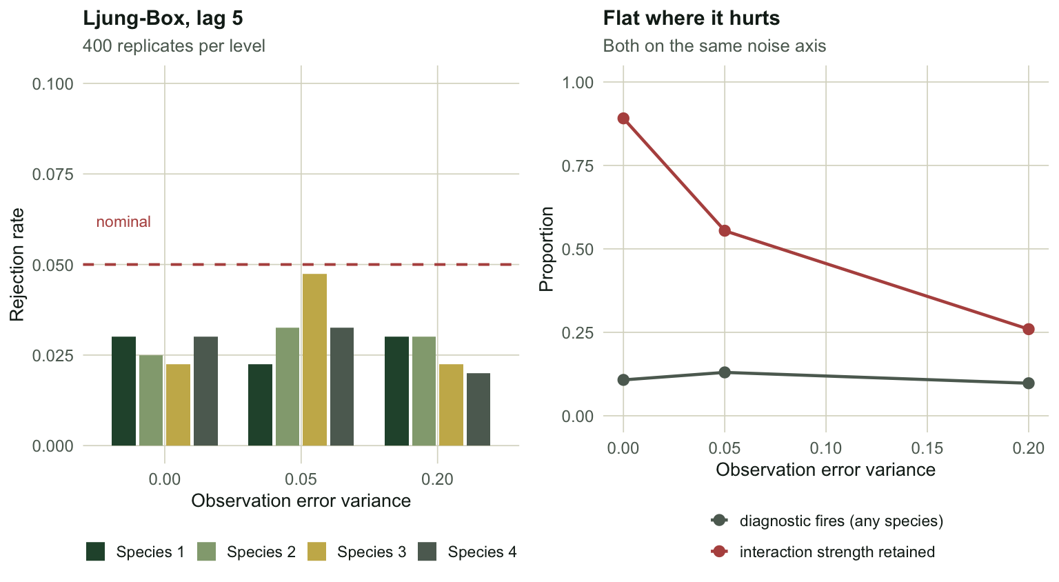
The natural defence is the residual check. A MAR(1) fit has residuals; if the model is wrong, the residuals should say so. Ljung-Box at lag 5 on each species, four hundred replicates, five per cent level.
```{r}
#| label: ljung-box
lb <- do.call(rbind, lapply(c(0, 0.05, 0.20), function(tau2) {
  rej <- matrix(FALSE, 400, p)
  for (m in 1:400) {
    Xt <- sim_mar1(60, Atrue, Btrue, Strue, seed = 300000 + m)
    set.seed(600000 + m)
    E <- mar1_cls(Xt + matrix(rnorm(60 * p, 0, sqrt(tau2)), 60, p))$E
    rej[m, ] <- sapply(1:p, function(i) Box.test(E[, i], lag = 5, type = "Ljung-Box")$p.value < 0.05)
  }
  data.frame(tau2 = tau2, sp1 = mean(rej[, 1]), sp2 = mean(rej[, 2]),
             sp3 = mean(rej[, 3]), sp4 = mean(rej[, 4]), any = mean(apply(rej, 1, any)))
}))
round(lb, 3)
```
At $\tau^2 = 0$ the test fires on `r sprintf("%.3f", round(lb$any[1], 3))` of replicates. That is below the `r sprintf("%.3f", 1 - 0.95^4)` four independent five per cent tests would give because Ljung-Box is conservative on residuals from a fitted model: the per-species rates sit near 0.03, and four independent tests at those rates would fire on about as many replicates as observed. At $\tau^2 = `r sprintf("%.2f", lb$tau2[3])`$, where the interaction matrix has collapsed by `r sprintf("%.0f", 100 - att$pct_of_truth[5])` per cent, the test fires on `r sprintf("%.3f", lb$any[3])`. If anything it fires slightly *less*.
The test sees nothing, at every noise level. That is not because the residuals are perfectly white: a state observed with error follows an ARMA(1,1) process, so the residuals of an AR(1) fit carry a small autocorrelation, but it is far too weak for Ljung-Box to find in sixty points. The damage attenuation does sits almost entirely in the rescaled coefficient, and a residual check is not built to see it. A model can be `r sprintf("%.0f", 100 - att$pct_of_truth[5])` per cent wrong about the quantity you care about and fail its residual check no more often than a correct model does.
```{r}
#| label: fig-silence
#| fig-width: 8
#| fig-height: 4.4
#| fig-cap: "Left: Ljung-Box rejection rates sit at or below the nominal level regardless of observation error. Right: the same information as a contrast, with the collapse of the interaction matrix on the same axis. The diagnostic is flat where the damage is steepest."
#| fig-alt: "Two panels. Left, bars of Ljung-Box rejection rate at three noise levels, all at or below the nominal five per cent line. Right, two lines against noise level: a flat one for the diagnostic and a steeply falling one for the retained interaction strength."
lbl <- do.call(rbind, lapply(1:nrow(lb), function(i) {
  data.frame(tau2 = factor(sprintf("%.2f", lb$tau2[i])),
             species = paste("Species", 1:4),
             rate = as.numeric(lb[i, c("sp1", "sp2", "sp3", "sp4")]))
}))

p1 <- ggplot(lbl, aes(tau2, rate, fill = species)) +
  geom_col(position = position_dodge(0.8), width = 0.7) +
  geom_hline(yintercept = 0.05, colour = te_rust, linetype = 2, linewidth = 0.7) +
  annotate("text", x = 0.7, y = 0.062, label = "nominal", colour = te_rust, size = 3) +
  scale_fill_manual(values = c(te_forest, te_sage, te_gold, te_muted)) +
  ylim(0, 0.1) +
  labs(title = "Ljung-Box, lag 5", subtitle = "400 replicates per level",
       x = "Observation error variance", y = "Rejection rate", fill = NULL) +
  theme_te(11)

cmp <- rbind(
  data.frame(tau2 = lb$tau2, v = lb$any, w = "diagnostic fires (any species)"),
  data.frame(tau2 = att$tau2[c(1, 3, 5)], v = att$pct_of_truth[c(1, 3, 5)] / 100,
             w = "interaction strength retained")
)

p2 <- ggplot(cmp, aes(tau2, v, colour = w)) +
  geom_line(linewidth = 0.8) +
  geom_point(size = 2.4) +
  scale_colour_manual(values = c(`diagnostic fires (any species)` = te_muted,
                                 `interaction strength retained` = te_rust)) +
  ylim(0, 1) +
  labs(title = "Flat where it hurts", subtitle = "Both on the same noise axis",
       x = "Observation error variance", y = "Proportion", colour = NULL) +
  theme_te(11) +
  guides(colour = guide_legend(ncol = 1))

two_panel(p1, p2)
```
## The mechanism is exact, and it is an old one
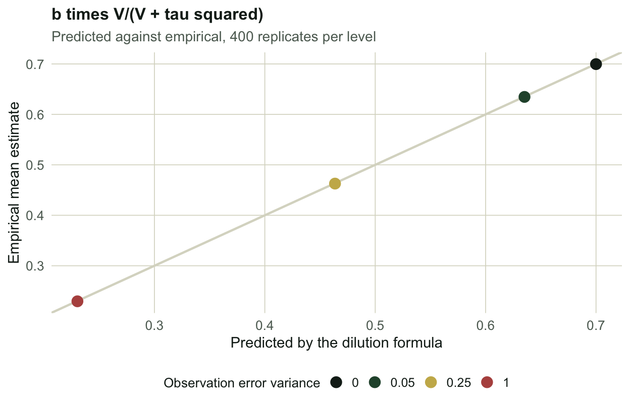
None of this is mysterious. Observation error in a MAR(1) model is measurement error in a *predictor*, because the lagged state is the predictor. That is regression dilution, and it has a closed form: the estimate converges to the truth times the reliability ratio.
$$\hat b \;\to\; b \cdot \frac{V}{V + \tau^2}$$
Check it at $p = 1$, where the algebra is clean, with long series so that small-sample bias is out of the way.
```{r}
#| label: reliability
b <- 0.7; s2 <- 0.25
V1 <- s2 / (1 - b^2)

rel <- do.call(rbind, lapply(c(0, 0.05, 0.25, 1.00), function(tau2) {
  bh <- numeric(400)
  for (m in 1:400) {
    set.seed(50000 + m)
    x <- numeric(3000)
    for (t in 2:3000) x[t] <- b * x[t - 1] + rnorm(1, 0, sqrt(s2))
    set.seed(150000 + m)
    xo <- x + rnorm(3000, 0, sqrt(tau2))
    bh[m] <- coef(lm(xo[-1] ~ xo[-3000]))[2]
  }
  data.frame(tau2 = tau2, empirical = mean(bh),
             predicted = b * V1 / (V1 + tau2),
             gap = mean(bh) - b * V1 / (V1 + tau2),
             reliability = V1 / (V1 + tau2))
}))
round(rel, 4)
```
The stationary variance is `r sprintf("%.4f", V1)`, and the formula predicts every row to within `r sprintf("%.4f", max(abs(rel$gap)))`. This is not an approximation that happens to work. It is the same reliability ratio as [Measurement error and regression dilution](../measurement-error-regression-dilution/), arriving in a time series because the lag makes the response into next step's predictor.
```{r}
#| label: fig-reliability
#| fig-width: 6.5
#| fig-height: 4.2
#| fig-cap: "The dilution formula against 400 simulations per noise level, at p = 1 with 3000-step series. The points sit on the line; the largest gap across the whole range is under 0.001."
#| fig-alt: "A scatter of empirical against predicted autoregressive coefficient for four noise levels, all four points lying on the one-to-one line running from about 0.23 up to 0.70."
ggplot(rel, aes(predicted, empirical)) +
  geom_abline(slope = 1, intercept = 0, colour = te_line, linewidth = 0.8) +
  geom_point(aes(colour = factor(tau2)), size = 3.4) +
  scale_colour_manual(values = c(te_ink, te_forest, te_gold, te_rust)) +
  labs(title = "b times V/(V + tau squared)",
       subtitle = "Predicted against empirical, 400 replicates per level",
       x = "Predicted by the dilution formula", y = "Empirical mean estimate",
       colour = "Observation error variance") +
  theme_te()
```
So the attenuation is not a bug to be diagnosed. It is the correct behaviour of least squares given a noisy predictor, and asking the residuals about it is asking the wrong question. The residuals describe the fit, and they look almost as they would without observation error. It is the *target* that moved.
## The remedy has to come from outside
The reliability ratio needs $\tau^2$, and a single short series pins $\tau^2$ down only weakly: its counts barely separate the wobble that is the community from the wobble that is your net. In practice something external has to supply it:
- **Repeated sampling within a time step.** Two hauls on the same day differ only by observation error, which estimates $\tau^2$ directly. This is the cleanest answer and it is a field-design decision, not an analysis decision.
- **A state-space model.** Put the latent true state and the observation layer in explicitly and let the Kalman filter separate them. [The Gompertz state-space model](../gompertz-state-space-model/) is the one-species version of exactly this, and `MARSS` (Holmes, Ward and Wills 2012) does the multivariate case.
The second option is the popular one, and it comes with its own honest limit that is worth knowing before you reach for it. The two variances are only weakly identified from a single series: Knape (2008) showed that for realistic parameter values the density dependence and the two error variances trade off against each other in a way one series cannot resolve, and Auger-Methe et al. (2016) found that even simple linear Gaussian state-space models hit parameter and state estimation problems more often than their popularity suggests. Dennis et al. (2006) is the careful treatment of the Gompertz case.
So the state-space model is not a machine that removes observation error. It is a machine that lets you *state* your assumption about observation error and propagate it honestly. If you have replicate samples, it works well. If you are hoping it will find $\tau^2$ for you out of sixty points, it may hand you a confident number that a slightly different starting value would have changed.
That is the same shape as every honest limit in this cluster: [the naive AR(1) shortcut](../fitting-a-mar1-model/) needs $\Sigma$ from outside, the [interaction estimates](../interaction-strengths-from-time-series/) need external information to break environmental synchrony, and the correction here needs $\tau^2$ from outside. A short series barely contains its own error rate.
## A checklist, and what it cannot cover
Before reporting a MAR(1) result:
1. **Series length.** Report it. Below about 100 points the diagonal carries visible small-sample bias, and the fix is arithmetic, not judgement.
2. **Observation error.** State what you assume $\tau^2$ is and where the assumption came from. "We assumed none" is a defensible answer only if you say it out loud, because it can set every stability metric too low.
3. **Environmental synchrony.** Check the VIF of the lagged design. Synchronised species have interactions that the data pin down only imprecisely, and no fitting method fixes that.
4. **Multiplicity.** A $p$-species fit tests $p^2$ cells. Control the false discovery rate before drawing the web.
5. **Residuals.** Run Ljung-Box, and understand that passing it rules out one narrow failure mode and nothing else.
The last item is the honest core of this post. Every check listed above is a falsification test: it can reject a model, and it can never confirm one. And the assumptions that matter most in a MAR(1) analysis are not on the list at all, because no diagnostic reaches them:
- **Linearity on the log scale.** MAR(1) is exactly right for Gompertz dynamics and a local approximation for anything else. Certain, Barraquand and Gardmark (2018) found the coefficients recover signs and ranks under nonlinear dynamics but not values, and the residuals do not complain.
- **No missing species.** An unmeasured species that drives two of your taxa shows up as an interaction between them. Nothing in the fit distinguishes that from the real thing.
- **Stationarity.** A community that is on its way somewhere has no stationary distribution for the return rate to be about.
A MAR(1) analysis that reports its series length, its observation-error assumption and its multiplicity correction, and that claims signs rather than strengths, is doing what the method supports. One that quotes a return rate to four decimals from sixty uncorrected counts is quoting the sampling protocol.
## References
- Ives AR, Dennis B, Cottingham KL, Carpenter SR 2003 Ecological Monographs 73(2):301-330 (10.1890/0012-9615(2003)073[0301:ECSAEI]2.0.CO;2)
- Dennis B, Ponciano JM, Lele SR, Taper ML, Staples DF 2006 Ecological Monographs 76(3):323-341 (10.1890/0012-9615(2006)76[323:EDDPNA]2.0.CO;2)
- Knape J 2008 Ecology 89(11):2994-3000 (10.1890/08-0071.1)
- Auger-Methe M, Field C, Albertsen CM, Derocher AE, Lewis MA, Jonsen ID, Mills Flemming J 2016 Scientific Reports 6:26677 (10.1038/srep26677)
- Holmes EE, Ward EJ, Wills K 2012 The R Journal 4(1):11-19 (10.32614/RJ-2012-002)
- Certain G, Barraquand F, Gardmark A 2018 Methods in Ecology and Evolution 9(9):1975-1995 (10.1111/2041-210X.13021)
## Related tutorials
- [Fitting a MAR(1) model to community time series](../fitting-a-mar1-model/)
- [Interaction strengths from community time series](../interaction-strengths-from-time-series/)
- [Community stability from a MAR(1) model](../stability-from-a-mar1-model/)
- [Observation error estimated as zero in a Gompertz fit](../observation-error-estimated-as-zero/)