---
title: "Community stability from a MAR(1) model"
description: "Turn a fitted interaction matrix into return rate, reactivity and variance ratios in base R, and see which stability reading survives more than one species."
date: "2026-06-11 10:00"
date-modified: "2026-10-07"
categories: [R, MAR models, stability, community ecology, ecology tutorial]
image: thumbnail.png
image-alt: "Four eigenvalues of an estimated interaction matrix on axes labelled real part and imaginary part, with a dashed circle drawn through the largest modulus of those estimates: a conjugate pair lies on the circle, two real eigenvalues fall inside it, and a solid vertical line marks the largest real part, which sits inside the circle's right edge rather than reaching it."
---
*Corrected 7 October 2026: the post read Ives's two reactivity summaries as agreeing that the community is not reactive, but one of them is negative for every stationary community and cannot say so; it also checked the return rate with a single step ratio taken while the transients were still large, and now takes it much later and says why the early decay runs a little faster than the dominant modulus.*
*Corrected 1 October 2026: the text description of the variance-ratio figure said all five bars differ in height and the dashed line for the determinant formula crosses them; the first two bars are equal and the line lies above every bar, and the description now says so.*
A fitted $B$ is not the point. The point is what it says about the community: how fast a perturbation decays, whether the community amplifies a shock before absorbing it, how much of the variation is environment rather than dynamics. Ives, Dennis, Cottingham and Carpenter (2003) laid out that toolkit, and every piece of it is a few lines of base R.
This post builds them from the definitions. Two of them have a trap in the implementation, and one of them means less than it looks like when you have more than one species.
```{r}
#| label: setup
#| code-fold: true
#| code-summary: "Setup: packages, colours and plot theme"
#| results: hide
#| message: false
#| warning: false
#| fig-show: hide
library(ggplot2)
library(grid)

te_ink    <- "#16241d"
te_forest <- "#275139"
te_gold   <- "#c9b458"
te_rust   <- "#b5534e"
te_sage   <- "#93a87f"
te_line   <- "#dad9ca"
te_muted  <- "#5d6b61"

theme_te <- function(base_size = 12) {
  theme_minimal(base_size = base_size) +
    theme(
      text             = element_text(colour = te_ink),
      plot.title       = element_text(face = "bold", size = rel(1.02), colour = te_ink),
      plot.subtitle    = element_text(colour = te_muted, size = rel(0.88)),
      axis.title       = element_text(colour = te_ink, size = rel(0.92)),
      axis.text        = element_text(colour = te_muted, size = rel(0.82)),
      panel.grid.major = element_line(colour = te_line, linewidth = 0.3),
      panel.grid.minor = element_blank(),
      panel.background = element_rect(fill = "#f5f4ee", colour = NA),
      plot.background  = element_rect(fill = "#f5f4ee", colour = NA),
      legend.position  = "bottom",
      legend.title     = element_text(size = rel(0.82)),
      legend.text      = element_text(size = rel(0.78)),
      legend.key.size  = unit(0.8, "lines")
    )
}

two_panel <- function(p1, p2) {
  grid.newpage()
  pushViewport(viewport(layout = grid.layout(1, 2)))
  print(p1, vp = viewport(layout.pos.row = 1, layout.pos.col = 1))
  print(p2, vp = viewport(layout.pos.row = 1, layout.pos.col = 2))
}

Btrue <- matrix(c( 0.50, -0.10, -0.35,  0.00,
                  -0.15,  0.60,  0.00,  0.00,
                   0.30,  0.00,  0.45, -0.30,
                   0.00,  0.00,  0.25,  0.55), 4, 4, byrow = TRUE)
Atrue <- c(1.20, 0.90, 0.40, 0.30)
Strue <- matrix(c(0.09, 0.03, 0, 0, 0.03, 0.09, 0, 0,
                  0, 0, 0.04, 0.01, 0, 0, 0.01, 0.04), 4, 4, byrow = TRUE)
p <- 4

sim_mar1 <- function(n, A, B, S, seed, burn = 200) {
  set.seed(seed); p <- length(A); L <- chol(S)
  x <- solve(diag(p) - B, A); X <- matrix(0, n, p)
  for (t in seq_len(burn + n)) {
    x <- A + B %*% x + as.vector(rnorm(p) %*% L)
    if (t > burn) X[t - burn, ] <- x
  }
  X
}
mar1_cls <- function(X) {
  n <- nrow(X); Y <- X[-1, , drop = FALSE]; D <- cbind(1, X[-n, , drop = FALSE])
  cf <- solve(crossprod(D), crossprod(D, Y)); E <- Y - D %*% cf
  list(A = cf[1, ], B = t(cf[-1, , drop = FALSE]), Sigma = crossprod(E) / nrow(Y), E = E)
}
```
```{r}
#| label: sci-tex-helper
#| include: false
sci_tex <- function(x, digits = 2) {
s <- formatC(x, format = "e", digits = digits)
paste0("$", sub("e.*", "", s), " \\times 10^{", as.integer(sub(".*e", "", s)), "}$")
}
```
## The stationary distribution, by hand
A stationary MAR(1) process wanders around a fixed mean with a fixed covariance. Both come out of $B$, $A$ and $\Sigma$ with no simulation at all.
The mean solves $\mu = A + B\mu$. The covariance solves the discrete Lyapunov equation $V = BVB' + \Sigma$, which vectorises into a plain linear system using the Kronecker product.
```{r}
#| label: stationary
stat_mu <- function(A, B) solve(diag(nrow(B)) - B, A)
stat_V  <- function(B, S) {
  matrix(solve(diag(nrow(B)^2) - kronecker(B, B), as.vector(S)), nrow(B), nrow(B))
}

Vt <- stat_V(Btrue, Strue)
round(Vt, 4)
```
Worth checking against brute force before trusting it anywhere else.
```{r}
#| label: stationary-check
Xlong <- sim_mar1(2e5, Atrue, Btrue, Strue, seed = 999)
max(abs(Vt - cov(Xlong)))
```
`r sprintf("%.4f", max(abs(Vt - cov(sim_mar1(2e5, Atrue, Btrue, Strue, seed = 999)))))` across all sixteen entries, against a two hundred thousand step simulation. The closed form is right, and it is instant.
## Return rate is the dominant eigenvalue modulus
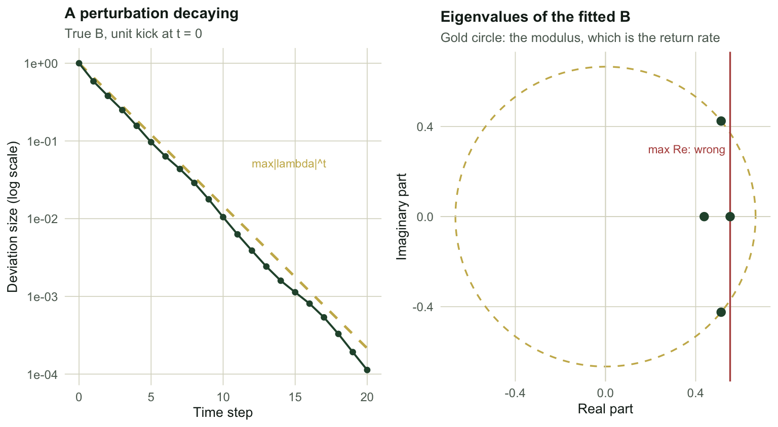
Kick the community away from equilibrium and the deviation evolves as $B^t z$. After the transients, the deviation shrinks by a constant factor each step, and that factor is the largest eigenvalue modulus of $B$.
```{r}
#| label: return-rate
set.seed(11)
z <- rnorm(p); z <- z / sqrt(sum(z^2))
for (t in 1:199) z <- as.vector(Btrue %*% z)
n199 <- sqrt(sum(z^2))
z <- as.vector(Btrue %*% z)
decay <- sqrt(sum(z^2)) / n199
c(empirical_decay = decay, max_eigen_mod = max(Mod(eigen(Btrue)$values)))
```
`r sprintf("%.4f", decay)` against `r sprintf("%.4f", max(Mod(eigen(Btrue)$values)))`. The perturbation really does decay at that rate once the transients have gone, but here they take a long time to go: a complex pair of eigenvalues has modulus `r sprintf("%.4f", sort(Mod(eigen(Btrue)$values), decreasing = TRUE)[2])`, close to the dominant one, so its share of the deviation fades slowly, and the check above takes the ratio only after many steps.
A community with a return rate near one takes forever to recover; near zero it snaps back in a step. This is the asymptotic resilience of the community, and it is the number most MAR(1) papers report.
## The trap: use the modulus, not the real part
`eigen()` on an asymmetric matrix returns complex numbers whenever the dominant pair spirals. Estimated interaction matrices do this constantly, even when the true matrix does not.
```{r}
#| label: complex-trap
fit <- mar1_cls(sim_mar1(60, Atrue, Btrue, Strue, seed = 4268))
ev  <- eigen(fit$B)$values
c(is_complex = is.complex(ev),
  max_modulus = max(Mod(ev)),
  max_real    = max(Re(ev)),
  truth       = max(Mod(eigen(Btrue)$values)))
```
The estimated matrix has a complex dominant pair. Its modulus is `r sprintf("%.4f", max(Mod(eigen(mar1_cls(sim_mar1(60, Atrue, Btrue, Strue, seed = 4268))$B)$values)))`, close to the truth of `r sprintf("%.4f", max(Mod(eigen(Btrue)$values)))`. Take the largest real part of any eigenvalue instead and you get `r sprintf("%.4f", max(Re(eigen(mar1_cls(sim_mar1(60, Atrue, Btrue, Strue, seed = 4268))$B)$values)))`, which belongs to a different, purely real eigenvalue and sits `r sprintf("%.0f", 100 * (1 - max(Re(eigen(mar1_cls(sim_mar1(60, Atrue, Btrue, Strue, seed = 4268))$B)$values)) / max(Mod(eigen(Btrue)$values))))` per cent below the truth.
`as.numeric()` on a complex vector silently keeps the real part and throws a warning about discarded imaginary parts. Code that wraps that call in `suppressWarnings()` is quietly reporting the wrong stability number for any community whose recovery oscillates. Use `max(Mod(...))`. When the return is a spiral rather than a slide, the modulus is the rate at which the spiral tightens, and the real part is not a decay rate at all.
The variance of the process returns at the square of that rate, which the Kronecker product confirms exactly.
```{r}
#| label: variance-return
max(Mod(eigen(kronecker(Btrue, Btrue))$values)) - max(Mod(eigen(Btrue)$values))^2
```
## Reactivity: stable communities can still amplify
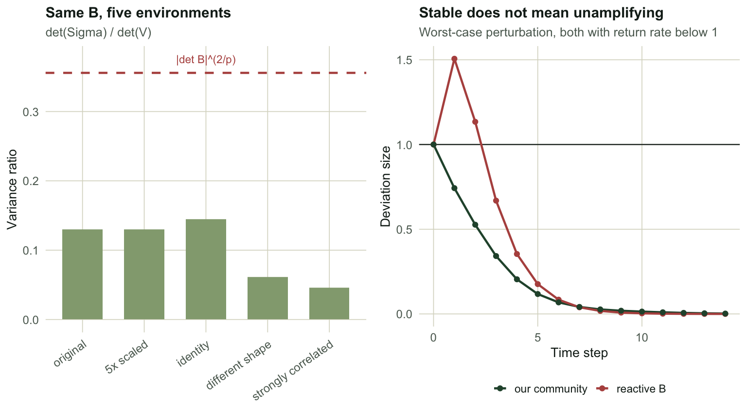
Asymptotic return rate says nothing about the first step. A perturbation can grow substantially before it decays, and Neubert and Caswell (1997) named that reactivity. The worst-case one-step amplification over all unit perturbations is the largest singular value of $B$.
```{r}
#| label: reactivity
sigma1 <- sqrt(max(eigen(crossprod(Btrue))$values))

set.seed(13)
amp <- replicate(2e5, {
  u <- rnorm(p); u <- u / sqrt(sum(u^2))
  sqrt(sum((Btrue %*% u)^2))
})
c(sigma1 = sigma1, brute_force_max = max(amp), gap = sigma1 - max(amp))
```
The algebra and two hundred thousand random directions agree to `r sci_tex(sigma1 - max(amp), 1)`. Our community has $\sigma_1 = `r sprintf("%.4f", sigma1)`$, below one, so no perturbation grows: it is not reactive. Ives's worst-case summary below, the largest eigenvalue of $B'B$ minus one, is $\sigma_1^2 - 1$ and so negative too. The other summary, minus the trace of $\Sigma$ over the trace of $V$, cannot settle the question: the Lyapunov equation makes the trace of $V$ the trace of $\Sigma$ plus that of $BVB'$, which is never negative, so this summary is negative for every stationary community, reactive or not.
```{r}
#| label: ives-reactivity
c(sigma_over_Vinf = -sum(diag(Strue)) / sum(diag(Vt)),
  worst_case      = max(eigen(crossprod(Btrue))$values) - 1)
```
Now a community that is stable and reactive at once, which is the case the eigenvalue misses entirely.
```{r}
#| label: reactive-example
Br <- matrix(c(0.4, 1.4,
               0,   0.4), 2, 2, byrow = TRUE)
c(return_rate = max(Mod(eigen(Br)$values)),
  sigma1      = sqrt(max(eigen(crossprod(Br))$values)))
```
Return rate `r sprintf("%.4f", max(Mod(eigen(matrix(c(0.4,1.4,0,0.4),2,2,byrow=TRUE))$values)))`, which is fast and comfortable. Largest singular value `r sprintf("%.4f", sqrt(max(eigen(crossprod(matrix(c(0.4,1.4,0,0.4),2,2,byrow=TRUE)))$values)))`, well above one. Some perturbations to this community grow by half again before they start shrinking. If your monitoring picks up the transient and not the asymptote, the return rate is the wrong summary to be quoting.
```{r}
#| label: fig-decay
#| fig-width: 8
#| fig-height: 4.4
#| fig-cap: "Left: a perturbation to the true community, with the dominant eigenvalue modulus to the power t as a dashed reference; over these early steps the transients have not died away, so it shrinks a little faster than the reference. Right: the eigenvalues of the estimated matrix in the complex plane. The dominant pair is complex, so its distance from the origin, not its horizontal position, is the return rate."
#| fig-alt: "Two panels. Left, a decaying curve of perturbation size against time step on a log scale, running just below a straight dashed reference line and slowly drifting further below it. Right, four points in the complex plane with a dashed circle through the outermost conjugate pair and a vertical line at the largest real part of any eigenvalue, which sits inside the circle's right edge rather than reaching it."
zz <- {
  set.seed(11); v <- rnorm(p); v <- v / sqrt(sum(v^2))
  out <- numeric(21); out[1] <- 1
  for (t in 2:21) { v <- as.vector(Btrue %*% v); out[t] <- sqrt(sum(v^2)) }
  out
}
lam <- max(Mod(eigen(Btrue)$values))
dec <- data.frame(t = 0:20, size = zz, ref = lam^(0:20))

p1 <- ggplot(dec, aes(t, size)) +
  geom_line(aes(y = ref), colour = te_gold, linewidth = 0.9, linetype = 2) +
  geom_line(colour = te_forest, linewidth = 0.7) +
  geom_point(colour = te_forest, size = 1.6) +
  scale_y_log10(labels = scales::label_log()) +
  annotate("text", x = 12, y = lam^7, label = "max|lambda|^t", colour = te_gold, size = 3, hjust = 0) +
  labs(title = "A perturbation decaying", subtitle = "True B, unit kick at t = 0",
       x = "Time step", y = "Deviation size (log scale)") +
  theme_te(11)

evd <- data.frame(re = Re(ev), im = Im(ev))
circ <- data.frame(a = seq(0, 2 * pi, length.out = 200))
circ$x <- max(Mod(ev)) * cos(circ$a); circ$y <- max(Mod(ev)) * sin(circ$a)

p2 <- ggplot(evd, aes(re, im)) +
  geom_path(data = circ, aes(x, y), colour = te_gold, linetype = 2, linewidth = 0.6) +
  geom_hline(yintercept = 0, colour = te_line, linewidth = 0.3) +
  geom_vline(xintercept = 0, colour = te_line, linewidth = 0.3) +
  geom_vline(xintercept = max(Re(ev)), colour = te_rust, linewidth = 0.6) +
  geom_point(colour = te_forest, size = 2.6) +
  annotate("text", x = max(Re(ev)) - 0.02, y = 0.3, label = "max Re: wrong",
           colour = te_rust, size = 3, hjust = 1) +
  coord_equal() +
  labs(title = "Eigenvalues of the fitted B",
       subtitle = "Gold circle: the modulus, which is the return rate",
       x = "Real part", y = "Imaginary part") +
  theme_te(11)

two_panel(p1, p2)
```
```{r}
#| label: thumb
#| include: false
thumb_title <- paste(strwrap("Eigenvalues of the fitted B", 46), collapse = "\n")
ggsave("thumbnail.png",
p2 + labs(title = thumb_title) +
theme(plot.title = element_text(size = 13, face = "bold"),
plot.subtitle = element_text(size = 9.5),
plot.margin = margin(8, 14, 8, 8)),
width = 7.5, height = 5.4, dpi = 100, bg = "#f5f4ee")
```
## The honest limit: what the variance ratio does not use
Ives et al. give a summary of stability as the proportion of the stationary variance attributable to environmental noise. At $p = 1$ it is an identity you can check on paper: the ratio $\Sigma/V$ is exactly $1 - b^2$. Since $|\det B|^{2/p}$ is just $b^2$ with one species, the noise share is $1 - |\det B|^{2/p}$, and the ratio itself generalises to the per-dimension form $[\det \Sigma / \det V]^{1/p}$.
```{r}
#| label: p1-identity
t(sapply(c(0.3, 0.7, 0.9), function(b) {
  V <- 0.25 / (1 - b^2)
  c(b = b, sigma_over_V = 0.25 / V, one_minus_b2 = 1 - b^2, gap = 0.25 / V - (1 - b^2))
}))
```
Exact to machine precision, and a clean reading: a species whose $b$ is near one has almost all of its variance built up by its own slow dynamics, and a species whose $b$ is near zero is just tracking the weather.
Now carry that reading to four species. Hold $B$ fixed and change only the shape of $\Sigma$.
```{r}
#| label: det-sweep
Sl <- list(
  "original"          = Strue,
  "5x scaled"         = 5 * Strue,
  "identity"          = diag(p) * 0.06,
  "different shape"   = diag(c(0.20, 0.02, 0.10, 0.01)),
  "strongly correlated" = 0.06 * (0.8 * matrix(1, p, p) + 0.2 * diag(p))
)
ratios <- sapply(Sl, function(S) (det(S) / det(stat_V(Btrue, S)))^(1 / p))
round(ratios, 6)
```
```{r}
#| label: det-b
c(det_B_2_over_p = abs(det(Btrue))^(2 / p),
  one_minus_it   = 1 - abs(det(Btrue))^(2 / p))
```
The actual variance ratio ranges from `r sprintf("%.6f", min(ratios))` to `r sprintf("%.6f", max(ratios))` across those five environments, a factor of `r sprintf("%.1f", max(ratios) / min(ratios))`. The formula $1 - |\det B|^{2/p}$ returns `r sprintf("%.6f", 1 - abs(det(Btrue))^(2/p))` for every one of them, because it does not contain $\Sigma$. It cannot vary with something it never reads.
Notice also that scaling $\Sigma$ by five changes nothing (`r sprintf("%.6f", ratios[["original"]])` both times): the ratio is scale invariant, so the disagreement is about the *shape* of the environmental covariance, not its size.
```{r}
#| label: fig-sigma
#| fig-width: 8
#| fig-height: 4.4
#| fig-cap: "Left: the true variance ratio moves with the shape of the environmental covariance while the determinant summary stays put, with B identical throughout. Right: a stable but reactive community, where the worst-case perturbation grows by half before it decays."
#| fig-alt: "Two panels. Left, five bars for the true variance ratio under five environments, the first two of equal height and the other three differing, all lying below a flat dashed line for the determinant formula. Right, a curve rising above one for two steps before decaying towards zero, against a comparison curve that never rises above one and decays steadily from the first step."
sw <- data.frame(env = factor(names(ratios), levels = names(ratios)),
                 ratio = as.vector(ratios))

p1 <- ggplot(sw, aes(env, ratio)) +
  geom_col(fill = te_sage, width = 0.65) +
  geom_hline(yintercept = 1 - abs(det(Btrue))^(2 / p), colour = te_rust,
             linetype = 2, linewidth = 0.8) +
  annotate("text", x = 3, y = 1 - abs(det(Btrue))^(2 / p) + 0.02,
           label = "1 - |det B|^(2/p)", colour = te_rust, size = 3) +
  labs(title = "Same B, five environments", subtitle = "(det Sigma / det V)^(1/p)",
       x = NULL, y = "Variance ratio") +
  theme_te(11) +
  theme(axis.text.x = element_text(angle = 35, hjust = 1))

amp_path <- function(B, steps = 14) {
  sv <- svd(B); v <- sv$v[, 1]
  out <- numeric(steps + 1); out[1] <- 1
  for (t in 1:steps) { v <- as.vector(B %*% v); out[t + 1] <- sqrt(sum(v^2)) }
  out
}
Br <- matrix(c(0.4, 1.4, 0, 0.4), 2, 2, byrow = TRUE)
react <- rbind(
  data.frame(t = 0:14, size = amp_path(Br), which = "reactive B"),
  data.frame(t = 0:14, size = amp_path(Btrue), which = "our community")
)

p2 <- ggplot(react, aes(t, size, colour = which)) +
  geom_hline(yintercept = 1, colour = te_ink, linewidth = 0.4) +
  geom_line(linewidth = 0.8) +
  geom_point(size = 1.5) +
  scale_colour_manual(values = c(`reactive B` = te_rust, `our community` = te_forest)) +
  labs(title = "Stable does not mean unamplifying",
       subtitle = "Worst-case perturbation, both with return rate below 1",
       x = "Time step", y = "Deviation size", colour = NULL) +
  theme_te(11)

two_panel(p1, p2)
```
So the one-species reading, "the fraction of variance that is environment rather than dynamics", does not carry to $p > 1$. That is a limit on the *interpretation*, not a fault in the framework: $|\det B|^{2/p}$ remains a perfectly good comparative index of how strongly the interaction matrix contracts, and Ives et al. present it as such. What it stops being, above one species, is a variance decomposition.
The general move is worth keeping. Before you accept an intuitive reading of a formula, look at which quantities appear in it. If the reading talks about something the formula never touches, the reading is borrowed from a special case.
## What to report
Return rate as $\max |\lambda(B)|$, computed with `Mod`. Reactivity as $\sigma_1(B)$, because a stable community can still amplify. The determinant index as a contraction summary, not as a variance share. And all of it conditional on $B$ being right, which [Checking a MAR(1) model](../checking-a-mar1-model/) is about: every number on this page inherits the estimation error in $B$, and the largest source of that error pushes all of them the same way.
If you suspect the community is not linear on the log scale to begin with, [The S-map and state-dependent dynamics](../s-map-and-state-dependence/) lets the local interaction matrix change with the state of the system, and MAR(1) is its globally linear special case.
## References
- Ives AR, Dennis B, Cottingham KL, Carpenter SR 2003 Ecological Monographs 73(2):301-330 (10.1890/0012-9615(2003)073[0301:ECSAEI]2.0.CO;2)
- Neubert MG, Caswell H 1997 Ecology 78(3):653-665 (10.1890/0012-9658(1997)078[0653:ATRFMT]2.0.CO;2)
- Hampton SE, Holmes EE, Scheef LP, Scheuerell MD, Katz SL, Pendleton DE, Ward EJ 2013 Ecology 94(12):2663-2669 (10.1890/13-0996.1)
- Certain G, Barraquand F, Gardmark A 2018 Methods in Ecology and Evolution 9(9):1975-1995 (10.1111/2041-210X.13021)
## Related tutorials
- [Fitting a MAR(1) model to community time series](../fitting-a-mar1-model/)
- [Interaction strengths from community time series](../interaction-strengths-from-time-series/)
- [Checking a MAR(1) model](../checking-a-mar1-model/)
- [Species synchrony and community stability](../synchrony-and-community-stability/)