---
title: "Fitting a MAR(1) model to community time series"
description: "Fit a multivariate autoregressive model to a plankton-like community in base R, and see why the single-species AR(1) shortcut answers a different question."
date: "2026-06-10 15:00"
date-modified: "2026-10-08"
categories: [R, MAR models, time series, community ecology, ecology tutorial]
image: thumbnail.png
image-alt: "Four simulated log-abundance series from a coupled four-species community, each in a brand colour."
---
*Corrected 8 October 2026: the section on the direction of the error was headed as if the shortcut always made a community look more stable; it is now headed as a result for this community, and it says that in another community off-diagonal feedback can lower the largest eigenvalue modulus, so that the diagonal alone overstates persistence.*
You have counted four plankton taxa every fortnight for a couple of years. You want the interaction matrix: who suppresses whom, and how hard. The first-order multivariate autoregressive model, MAR(1), is the standard answer to that question in community ecology, and the machinery behind it is about three lines of base R.
This post fits one from scratch. The fitting turns out to be the easy part. The interesting part is what happens when you skip it and fit a separate AR(1) to each species instead, which is what most people reach for first.
```{r}
#| label: setup
#| code-fold: true
#| code-summary: "Setup: packages, colours and plot theme"
#| results: hide
#| message: false
#| warning: false
#| fig-show: hide
library(ggplot2)
library(grid)

te_ink    <- "#16241d"
te_forest <- "#275139"
te_gold   <- "#c9b458"
te_rust   <- "#b5534e"
te_sage   <- "#93a87f"
te_line   <- "#dad9ca"
te_muted  <- "#5d6b61"

theme_te <- function(base_size = 12) {
  theme_minimal(base_size = base_size) +
    theme(
      text             = element_text(colour = te_ink),
      plot.title       = element_text(face = "bold", size = rel(1.02), colour = te_ink),
      plot.subtitle    = element_text(colour = te_muted, size = rel(0.88)),
      axis.title       = element_text(colour = te_ink, size = rel(0.92)),
      axis.text        = element_text(colour = te_muted, size = rel(0.82)),
      panel.grid.major = element_line(colour = te_line, linewidth = 0.3),
      panel.grid.minor = element_blank(),
      panel.background = element_rect(fill = "#f5f4ee", colour = NA),
      plot.background  = element_rect(fill = "#f5f4ee", colour = NA),
      legend.position  = "bottom",
      legend.title     = element_text(size = rel(0.82)),
      legend.text      = element_text(size = rel(0.78)),
      legend.key.size  = unit(0.8, "lines")
    )
}

two_panel <- function(p1, p2) {
  grid.newpage()
  pushViewport(viewport(layout = grid.layout(1, 2)))
  print(p1, vp = viewport(layout.pos.row = 1, layout.pos.col = 1))
  print(p2, vp = viewport(layout.pos.row = 1, layout.pos.col = 2))
}
```
## The model
Write $X_t$ for the vector of log abundances of $p$ species at time $t$. The MAR(1) process is
$$X_t = A + B\,X_{t-1} + E_t, \qquad E_t \sim \mathrm{MVN}(0, \Sigma).$$
Three objects carry the ecology. $A$ is a vector of intrinsic growth terms. $B$ is the $p \times p$ interaction matrix: $b_{ij}$ is the effect of species $j$'s log abundance on species $i$'s per-capita growth rate. $\Sigma$ is the covariance of the environmental shocks, which is where shared weather, shared sampling error and everything else the model does not name ends up.
The log scale is not decoration. On the log scale a Gompertz competition model is exactly linear, so MAR(1) is either a literal Gompertz community model or a linear approximation to something nonlinear near its equilibrium. Which of those you mean matters later; for now the algebra is the same.
## A community to fit
Four taxa, with a mix of strong and weak links and six true zeros. Two of them share a strongly correlated environment later on, but that second covariance matrix waits until we get there; the baseline one is below.
```{r}
#| label: dgp
Btrue <- matrix(c( 0.50, -0.10, -0.35,  0.00,
                  -0.15,  0.60,  0.00,  0.00,
                   0.30,  0.00,  0.45, -0.30,
                   0.00,  0.00,  0.25,  0.55), 4, 4, byrow = TRUE)
Atrue <- c(1.20, 0.90, 0.40, 0.30)
Strue <- matrix(c(0.09, 0.03, 0,    0,
                  0.03, 0.09, 0,    0,
                  0,    0,    0.04, 0.01,
                  0,    0,    0.01, 0.04), 4, 4, byrow = TRUE)
p <- 4

sim_mar1 <- function(n, A, B, S, seed, burn = 200) {
  set.seed(seed)
  p <- length(A)
  L <- chol(S)
  x <- solve(diag(p) - B, A)          # start at the stationary mean
  X <- matrix(0, n, p)
  for (t in seq_len(burn + n)) {
    x <- A + B %*% x + as.vector(rnorm(p) %*% L)
    if (t > burn) X[t - burn, ] <- x
  }
  X
}

X <- sim_mar1(60, Atrue, Btrue, Strue, seed = 4268)
```
There is no `MASS` here: `chol(S)` plus `rnorm` draws correlated normals in one line. The process is stationary because the largest eigenvalue modulus of $B$ is `r sprintf("%.4f", max(Mod(eigen(Btrue)$values)))`, comfortably below one.
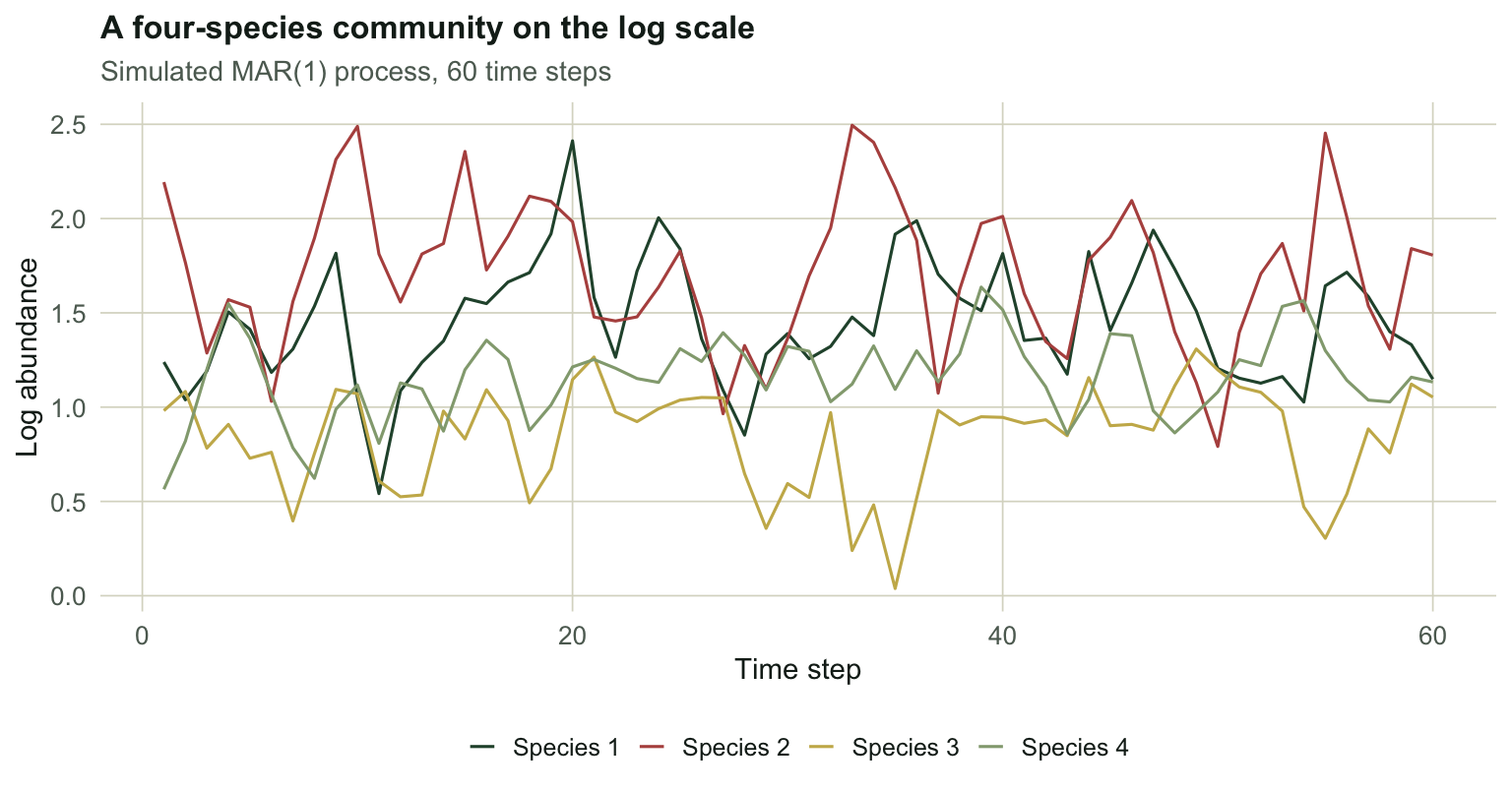
Sixty fortnights is a realistic length for a monitoring series, and short enough to be honest about.
```{r}
#| label: fig-series
#| fig-width: 8
#| fig-height: 4.2
#| fig-cap: "Sixty time steps of log abundance for the four simulated taxa. All four are stationary, all four wander, and nothing about the picture says which species is pushing which."
#| fig-alt: "Four coloured lines showing log abundance over sixty time steps for species one to four, each fluctuating around its own level without visible trend."
series <- data.frame(
  time    = rep(seq_len(nrow(X)), 4),
  logabun = as.vector(X),
  species = factor(rep(paste("Species", 1:4), each = nrow(X)))
)

ggplot(series, aes(time, logabun, colour = species)) +
  geom_line(linewidth = 0.55) +
  scale_colour_manual(values = c(te_forest, te_rust, te_gold, te_sage)) +
  labs(title = "A four-species community on the log scale",
       subtitle = "Simulated MAR(1) process, 60 time steps",
       x = "Time step", y = "Log abundance", colour = NULL) +
  theme_te()
```
## Fitting it: three lines
Conditional least squares stacks each time step's response on the previous step's state and solves the normal equations once.
```{r}
#| label: fit
mar1_cls <- function(X) {
  n  <- nrow(X)
  Y  <- X[-1, , drop = FALSE]           # response: steps 2..n
  D  <- cbind(1, X[-n, , drop = FALSE]) # design: intercept + steps 1..n-1
  cf <- solve(crossprod(D), crossprod(D, Y))
  E  <- Y - D %*% cf
  list(A = cf[1, ], B = t(cf[-1, , drop = FALSE]),
       Sigma = crossprod(E) / nrow(Y), E = E)
}

fit <- mar1_cls(X)
round(fit$B, 3)
```
That is the whole estimator. The transpose on the way out is the only fiddly bit: `cf` comes back with predictors in rows and responses in columns, and $B$ is indexed the other way round.
Standard errors come per cell from the usual least-squares algebra.
```{r}
#| label: se
mar1_se <- function(X) {
  n <- nrow(X); pp <- ncol(X)
  Y <- X[-1, , drop = FALSE]
  D <- cbind(1, X[-n, , drop = FALSE])
  XtXi <- solve(crossprod(D))
  q <- nrow(Y); k <- ncol(D)
  SE <- matrix(0, pp, pp)
  for (i in 1:pp) {
    r <- Y[, i] - D %*% (XtXi %*% crossprod(D, Y[, i]))
    SE[i, ] <- sqrt(sum(r^2) / (q - k) * diag(XtXi))[-1]
  }
  SE
}

SE <- mar1_se(X)
round(SE, 3)
```
## The multivariate fit is p separate regressions
Here is the thing that is worth knowing before you write anything about $B$. Fit species 1's row with `lm`, species 2's row with `lm`, and so on, ignoring the other species entirely while you do it. Compare.
```{r}
#| label: cls-is-ols
lmB <- t(sapply(1:p, function(i) coef(lm(X[-1, i] ~ X[-nrow(X), ]))[-1]))
max(abs(fit$B - lmB))
```
The largest difference printed above is floating-point rounding. Not close: identical.
The reason is a result older than MAR models. Every equation in the system uses the *same* design matrix, the lagged state of all species. When the regressors are identical across equations, generalised least squares collapses to equation-by-equation ordinary least squares, and the cross-equation error correlation buys you nothing (Zellner 1962). MAR(1) is a seemingly unrelated regression system in its degenerate case.
Two consequences follow, and they pull in opposite directions.
The comfortable one: the per-cell OLS standard errors above are valid, and you can reason about each row on its own.
The uncomfortable one: the "multivariate" in multivariate autoregressive does no work in estimating $B$. The multivariate part lives entirely in $\Sigma$, and $\Sigma$ is not something the fit uses to find $B$; it is something the fit reports afterwards. Every claim you make about $\Sigma$ mattering has to be a claim about something other than the point estimates of $B$.
## Does it recover the truth?
At $n = 60$ the estimates are noisy but sane. With a long enough series they converge.
```{r}
#| label: consistency
Xlong <- sim_mar1(4000, Atrue, Btrue, Strue, seed = 4001)
rbind(true = diag(Btrue), n60 = diag(fit$B), n4000 = diag(mar1_cls(Xlong)$B))
```
```{r}
#| label: fig-recovery
#| fig-width: 8
#| fig-height: 4.4
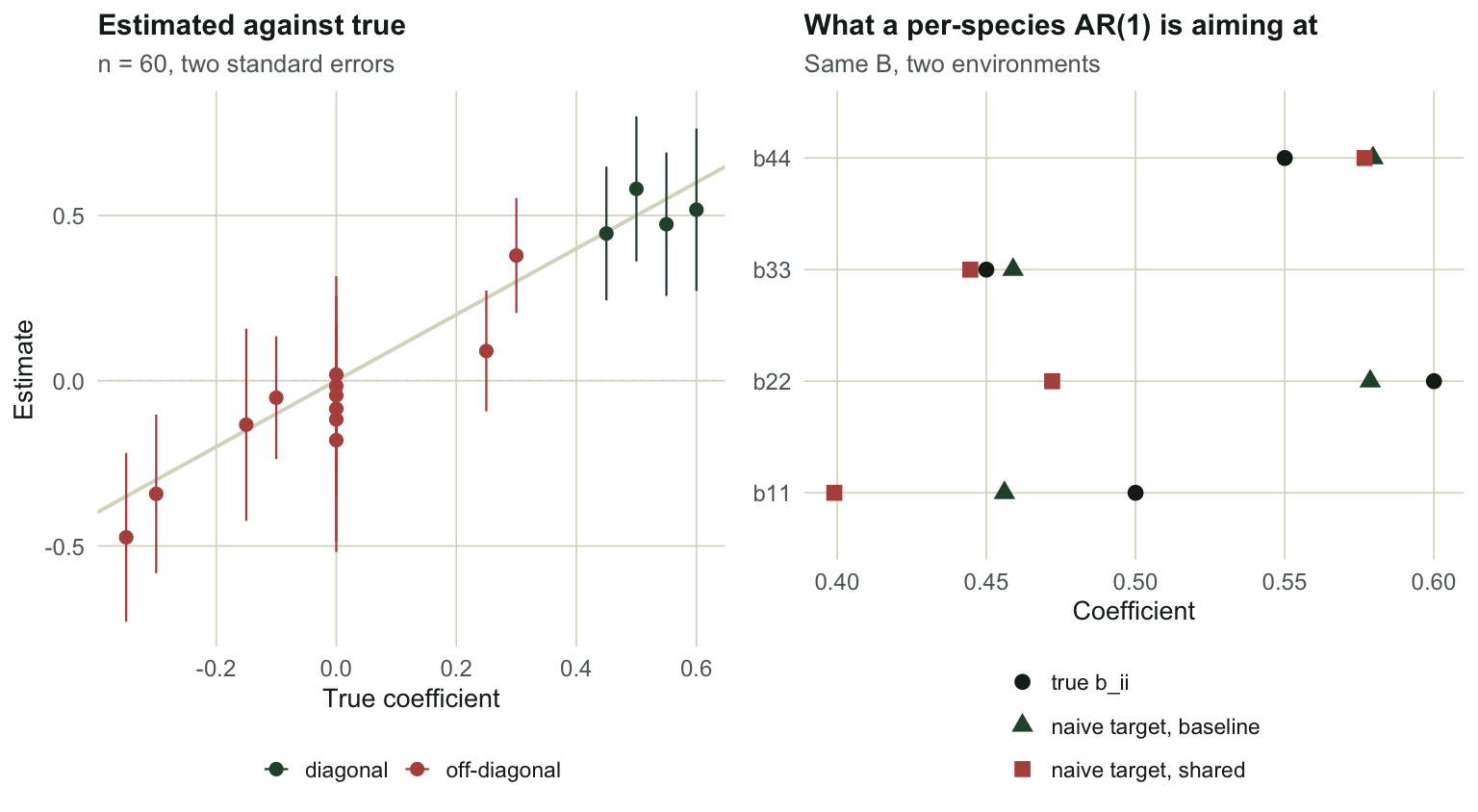
#| fig-cap: "Left: all sixteen estimated interaction coefficients against their true values, with two standard errors. Right: what a per-species AR(1) converges to, under two environments that share the same B. The naive answer moves; B did not."
#| fig-alt: "Two panels. Left, a scatter of estimated against true interaction coefficients scattered around the one-to-one line with error bars. Right, a dot plot comparing true diagonal coefficients with the naive AR(1) target under baseline and shared environments, the shared-environment points sitting to the left of the baseline points."
stat_V <- function(B, S) {
  matrix(solve(diag(nrow(B)^2) - kronecker(B, B), as.vector(S)), nrow(B), nrow(B))
}
naive_target <- function(B, S) { V <- stat_V(B, S); diag(B %*% V) / diag(V) }

Scol <- Strue; Scol[1, 2] <- Scol[2, 1] <- 0.087

rec <- data.frame(
  true = as.vector(Btrue), est = as.vector(fit$B), se = as.vector(SE),
  kind = ifelse(as.vector(diag(4)) == 1, "diagonal", "off-diagonal")
)

p1 <- ggplot(rec, aes(true, est, colour = kind)) +
  geom_abline(slope = 1, intercept = 0, colour = te_line, linewidth = 0.7) +
  geom_hline(yintercept = 0, colour = te_line, linewidth = 0.3, linetype = 3) +
  geom_errorbar(aes(ymin = est - 2 * se, ymax = est + 2 * se), width = 0, linewidth = 0.4) +
  geom_point(size = 2) +
  scale_colour_manual(values = c(diagonal = te_forest, `off-diagonal` = te_rust)) +
  labs(title = "Estimated against true", subtitle = "n = 60, two standard errors",
       x = "True coefficient", y = "Estimate", colour = NULL) +
  theme_te(11)

nv <- data.frame(
  species = rep(paste0("b", 1:4, 1:4), 3),
  value   = c(diag(Btrue), naive_target(Btrue, Strue), naive_target(Btrue, Scol)),
  what    = rep(c("true b_ii", "naive target, baseline", "naive target, shared"), each = 4)
)
nv$what <- factor(nv$what, levels = c("true b_ii", "naive target, baseline", "naive target, shared"))

p2 <- ggplot(nv, aes(value, species, colour = what, shape = what)) +
  geom_point(size = 2.6) +
  scale_colour_manual(values = c(te_ink, te_forest, te_rust)) +
  scale_shape_manual(values = c(16, 17, 15)) +
  labs(title = "What a per-species AR(1) is aiming at",
       subtitle = "Same B, two environments",
       x = "Coefficient", y = NULL, colour = NULL, shape = NULL) +
  theme_te(11) +
  guides(colour = guide_legend(ncol = 1), shape = guide_legend(ncol = 1))

two_panel(p1, p2)
```
At `r nrow(Xlong)` steps the diagonal comes back as `r paste(sprintf("%.4f", diag(mar1_cls(Xlong)$B)), collapse = ", ")` against a truth of `r paste(sprintf("%.2f", diag(Btrue)), collapse = ", ")`. The estimator is consistent. Sixty points is simply not four thousand.
## The shortcut, and what it actually estimates
Now the part that sends most people wrong. Fitting a separate AR(1) to each species is easy, needs no matrix algebra, and gives you a number per species that looks like $b_{ii}$. It is tempting to call the difference "bias" and move on.
It is not bias. A per-species AR(1) regresses $X_{i,t}$ on $X_{i,t-1}$ alone, so it converges on the population regression coefficient of one on the other, which is $(BV)_{ii}/V_{ii}$ where $V$ is the stationary covariance of the process. That quantity is a perfectly well-defined thing. It is just not $b_{ii}$.
```{r}
#| label: naive-target
rbind(`true b_ii`  = diag(Btrue),
      `naive aims at` = naive_target(Btrue, Strue))
```
The gap is small here. Now change nothing about the ecology. Keep $B$ exactly as it is, and only make species 1 and 2 share their environment, taking their shock correlation from `r sprintf("%.2f", Strue[1,2]/sqrt(Strue[1,1]*Strue[2,2]))` to `r sprintf("%.3f", Scol[1,2]/sqrt(Scol[1,1]*Scol[2,2]))`.
```{r}
#| label: naive-shared
Va <- stat_V(Btrue, Strue); Vc <- stat_V(Btrue, Scol)
rbind(`true b_ii`  = diag(Btrue),
      baseline     = naive_target(Btrue, Strue),
      shared       = naive_target(Btrue, Scol))
c(cor_baseline = Va[1, 2] / sqrt(Va[1, 1] * Va[2, 2]),
  cor_shared   = Vc[1, 2] / sqrt(Vc[1, 1] * Vc[2, 2]))
```
The observed correlation between species 1 and 2 goes from `r sprintf("%.3f", Va[1,2]/sqrt(Va[1,1]*Va[2,2]))` to `r sprintf("%.3f", Vc[1,2]/sqrt(Vc[1,1]*Vc[2,2]))`, and the naive answer for species 1 moves from `r sprintf("%.4f", naive_target(Btrue, Strue)[1])` to `r sprintf("%.4f", naive_target(Btrue, Scol)[1])`, a shift of `r sprintf("%.3f", naive_target(Btrue, Strue)[1] - naive_target(Btrue, Scol)[1])`. Species 2 moves by `r sprintf("%.3f", naive_target(Btrue, Strue)[2] - naive_target(Btrue, Scol)[2])`. The interaction matrix is byte-for-byte the same in both runs. Only $\Sigma$ changed.
This is the point of the whole exercise. The per-species AR(1) is a consistent estimator of a quantity that mixes $B$ with $\Sigma$. If two lakes give you different single-species density dependence, that difference can be entirely environmental correlation, with identical species interactions in both.
Before you write the word "bias" about any shortcut estimator, work out what it is consistent for. Sometimes the shortcut is consistent for the wrong thing, and that is worse than being biased for the right one, because nothing in the output complains. In a series as short as this one the shortcut is also biased towards zero on top of that, the usual small-sample behaviour of an autoregression.
## The direction of the error in this community
Feed the naive diagonal into the community's return rate, which is the largest eigenvalue modulus of the interaction matrix. Two things go wrong there, and only one of them is the estimator's fault. A diagonal matrix has no off-diagonal feedback, so its largest eigenvalue modulus is just its largest entry in absolute value: the exact true diagonal would already give `r sprintf("%.2f", max(abs(diag(Btrue))))`, short of what the full $B$ gives. That is a property of this $B$ and not a rule: in another community off-diagonal feedback can instead lower the largest modulus, and then the diagonal alone overstates persistence. Here what the naive estimator gets wrong about $b_{ii}$ happens to move it a little further down, although some of the naive targets sit above their true values.
```{r}
#| label: naive-stability
c(naive_baseline = max(Mod(eigen(diag(naive_target(Btrue, Strue)))$values)),
  naive_shared   = max(Mod(eigen(diag(naive_target(Btrue, Scol)))$values)),
  truth          = max(Mod(eigen(Btrue)$values)))
```
True return rate `r sprintf("%.4f", max(Mod(eigen(Btrue)$values)))`; the naive diagonal says `r sprintf("%.4f", max(Mod(eigen(diag(naive_target(Btrue, Strue)))$values)))` in the baseline environment and `r sprintf("%.4f", max(Mod(eigen(diag(naive_target(Btrue, Scol)))$values)))` in the shared one. Both understate persistence, which is to say both make the community look more stable than it is. That is the comfortable direction of error, and it is the direction the shortcut takes in both environments. [Checking a MAR(1) model](../checking-a-mar1-model/) shows a second, larger mechanism pushing the same way.
## The honest limit
The gap between the naive answer and $b_{ii}$ is set by $\Sigma$, and $\Sigma$ is exactly what a per-species analysis never sees. So the honest statement is not "the shortcut is off by about 0.05". It is: the size of the gap depends on the covariance structure, and without fitting the full model you have no way of knowing which case you are in.
That is a good reason to fit the model even when you only care about one species.
Two limits belong to the full model too. MAR(1) assumes linearity on the log scale, and when the underlying dynamics are nonlinear the coefficients recover signs and ranks far more reliably than values (Certain, Barraquand and Gardmark 2018). And it assumes the species you left out do not matter, which no amount of data will tell you.
## Where to go next
[Interaction strengths from community time series](../interaction-strengths-from-time-series/) takes the off-diagonal seriously: what the coefficients mean, how badly a 60-point series estimates them, and what shared environments do to their precision. [Community stability from a MAR(1) model](../stability-from-a-mar1-model/) turns $B$ into stability metrics by hand. If you suspect the log-linear assumption is doing too much work, [The S-map and state-dependent dynamics](../s-map-and-state-dependence/) is the state-dependent generalisation of the same idea: MAR(1) is the globally linear special case.
For a real analysis, the `MARSS` package fits this model class with observation error included (Holmes, Ward and Wills 2012), and Hampton et al. (2013) is the ecological review to start from.
## References
- Ives A R, Dennis B, Cottingham K L, Carpenter S R 2003 Ecological Monographs 73(2):301-330 (10.1890/0012-9615(2003)073[0301:ECSAEI]2.0.CO;2)
- Zellner A 1962 Journal of the American Statistical Association 57(298):348-368 (10.1080/01621459.1962.10480664)
- Hampton S E, Holmes E E, Scheef L P, Scheuerell M D, Katz S L, Pendleton D E, Ward E J 2013 Ecology 94(12):2663-2669 (10.1890/13-0996.1)
- Holmes E E, Ward E J, Wills K 2012 The R Journal 4(1):11-19 (10.32614/RJ-2012-002)
- Certain G, Barraquand F, Gardmark A 2018 Methods in Ecology and Evolution 9(9):1975-1995 (10.1111/2041-210X.13021)
## Related tutorials
- [Interaction strengths from community time series](../interaction-strengths-from-time-series/)
- [Community stability from a MAR(1) model](../stability-from-a-mar1-model/)
- [Checking a MAR(1) model](../checking-a-mar1-model/)
- [The Gompertz state-space model](../gompertz-state-space-model/)