---
title: "Interaction strengths from community time series"
description: "What a MAR(1) coefficient means, how much a sixty-point series can say about it, and why shared weather blurs the estimated effects of synchronised species."
date: "2026-06-11 09:00"
date-modified: "2026-10-14"
categories: [R, MAR models, time series, species interactions, ecology tutorial]
image: thumbnail.png
image-alt: "Estimation bias per cell of a four-species interaction matrix, with diagonal cells biased downwards and off-diagonal cells centred."
---
*Corrected 14 October 2026: the post compared the diagonal bias with a signed average of the off-diagonal biases, in which cells of opposite sign cancel, and said the direct interactions do not look stronger than they are; it now compares mean absolute biases and says most direct interactions look slightly stronger; and a section heading no longer says weak links are worse than absent.*
*Corrected 7 October 2026: the post said the small-sample bias lands on the diagonal whatever the parameters, and now says it does so here but partly moves into an interaction in the shared environment; it said one run in five would call the weak competitor a mutualist, and now adds that almost none of those wrong-signed estimates pass the screen; and the description no longer says a shared environment ruins the off-diagonal estimates.*
*Corrected 30 September 2026: the post said a shared environment breaks identifiability, that the data could no longer separate the interaction from the shared response, and called this fatal; it now says the coefficients stay identified but are estimated much less precisely.*
Fit a MAR(1) model and you get sixteen numbers for a four-species community. [Fitting a MAR(1) model to community time series](../fitting-a-mar1-model/) showed the fitting is three lines of base R and that the estimator is consistent. Consistent is a statement about infinite data. This post asks what sixty points buy you.
The answer has three parts, and only the first is the one people expect.
```{r}
#| label: setup
#| code-fold: true
#| code-summary: "Setup: packages, colours and plot theme"
#| results: hide
#| message: false
#| warning: false
#| fig-show: hide
library(ggplot2)
library(grid)

te_ink    <- "#16241d"
te_forest <- "#275139"
te_gold   <- "#c9b458"
te_rust   <- "#b5534e"
te_sage   <- "#93a87f"
te_line   <- "#dad9ca"
te_muted  <- "#5d6b61"

theme_te <- function(base_size = 12) {
  theme_minimal(base_size = base_size) +
    theme(
      text             = element_text(colour = te_ink),
      plot.title       = element_text(face = "bold", size = rel(1.02), colour = te_ink),
      plot.subtitle    = element_text(colour = te_muted, size = rel(0.88)),
      axis.title       = element_text(colour = te_ink, size = rel(0.92)),
      axis.text        = element_text(colour = te_muted, size = rel(0.82)),
      panel.grid.major = element_line(colour = te_line, linewidth = 0.3),
      panel.grid.minor = element_blank(),
      panel.background = element_rect(fill = "#f5f4ee", colour = NA),
      plot.background  = element_rect(fill = "#f5f4ee", colour = NA),
      legend.position  = "bottom",
      legend.title     = element_text(size = rel(0.82)),
      legend.text      = element_text(size = rel(0.78)),
      legend.key.size  = unit(0.8, "lines")
    )
}

two_panel <- function(p1, p2) {
  grid.newpage()
  pushViewport(viewport(layout = grid.layout(1, 2)))
  print(p1, vp = viewport(layout.pos.row = 1, layout.pos.col = 1))
  print(p2, vp = viewport(layout.pos.row = 1, layout.pos.col = 2))
}

Btrue <- matrix(c( 0.50, -0.10, -0.35,  0.00,
                  -0.15,  0.60,  0.00,  0.00,
                   0.30,  0.00,  0.45, -0.30,
                   0.00,  0.00,  0.25,  0.55), 4, 4, byrow = TRUE)
Atrue <- c(1.20, 0.90, 0.40, 0.30)
Strue <- matrix(c(0.09, 0.03, 0, 0, 0.03, 0.09, 0, 0,
                  0, 0, 0.04, 0.01, 0, 0, 0.01, 0.04), 4, 4, byrow = TRUE)
Scol  <- Strue; Scol[1, 2] <- Scol[2, 1] <- 0.087
p <- 4

sim_mar1 <- function(n, A, B, S, seed, burn = 200) {
  set.seed(seed); p <- length(A); L <- chol(S)
  x <- solve(diag(p) - B, A); X <- matrix(0, n, p)
  for (t in seq_len(burn + n)) {
    x <- A + B %*% x + as.vector(rnorm(p) %*% L)
    if (t > burn) X[t - burn, ] <- x
  }
  X
}
mar1_cls <- function(X) {
  n <- nrow(X); Y <- X[-1, , drop = FALSE]; D <- cbind(1, X[-n, , drop = FALSE])
  cf <- solve(crossprod(D), crossprod(D, Y)); E <- Y - D %*% cf
  list(A = cf[1, ], B = t(cf[-1, , drop = FALSE]), Sigma = crossprod(E) / nrow(Y), E = E)
}
mar1_se <- function(X) {
  n <- nrow(X); pp <- ncol(X); Y <- X[-1, , drop = FALSE]; D <- cbind(1, X[-n, , drop = FALSE])
  XtXi <- solve(crossprod(D)); q <- nrow(Y); k <- ncol(D); SE <- matrix(0, pp, pp)
  for (i in 1:pp) {
    r <- Y[, i] - D %*% (XtXi %*% crossprod(D, Y[, i]))
    SE[i, ] <- sqrt(sum(r^2) / (q - k) * diag(XtXi))[-1]
  }
  SE
}
```
## What the coefficients mean
$b_{ij}$ for $i \neq j$ is the effect of species $j$ on species $i$'s per-capita growth rate, per unit of log abundance. Negative means suppression, positive means facilitation, zero means no direct link. The sign convention is the ecologist's, so a competitor sits at a negative off-diagonal.
The diagonal is a different animal. $b_{ii}$ measures density dependence, and the useful way to read it is as persistence:
- $b_{ii} = 1$: no density dependence at all. A shock never decays and the species does a random walk.
- $b_{ii} = 0.9$: strong persistence, slow return, long memory of the last bad winter.
- $b_{ii} = 0$: total density dependence. Whatever happened last time step is gone; the species snaps straight back to its mean.
- $b_{ii} < 0$: overcompensation, the boom-and-bust of an overshooting population.
So the diagonal and the off-diagonal are not two flavours of the same number. One is a memory length, the other is a direct effect.
## The bias is asymmetric
Simulate the same community 600 times at $n = 60$ and average the estimates.
```{r}
#| label: mc
mc <- function(n, S, M, seed0) {
  Bh <- array(0, c(M, p, p)); Sg <- array(0, c(M, p, p))
  for (m in 1:M) {
    Xm <- sim_mar1(n, Atrue, Btrue, S, seed = seed0 + m)
    f <- mar1_cls(Xm)
    Bh[m, , ] <- f$B
    Sg[m, , ] <- abs(f$B / mar1_se(Xm)) > 2   # crude 2-SE screen
  }
  list(B = Bh, sig = Sg)
}

r60  <- mc(60, Strue, 600, 60000)
bias <- apply(r60$B, c(2, 3), mean) - Btrue
round(bias, 3)
```
```{r}
#| label: bias-split
c(diagonal     = mean(diag(bias)),
  off_diagonal = mean(bias[row(bias) != col(bias)]))
```
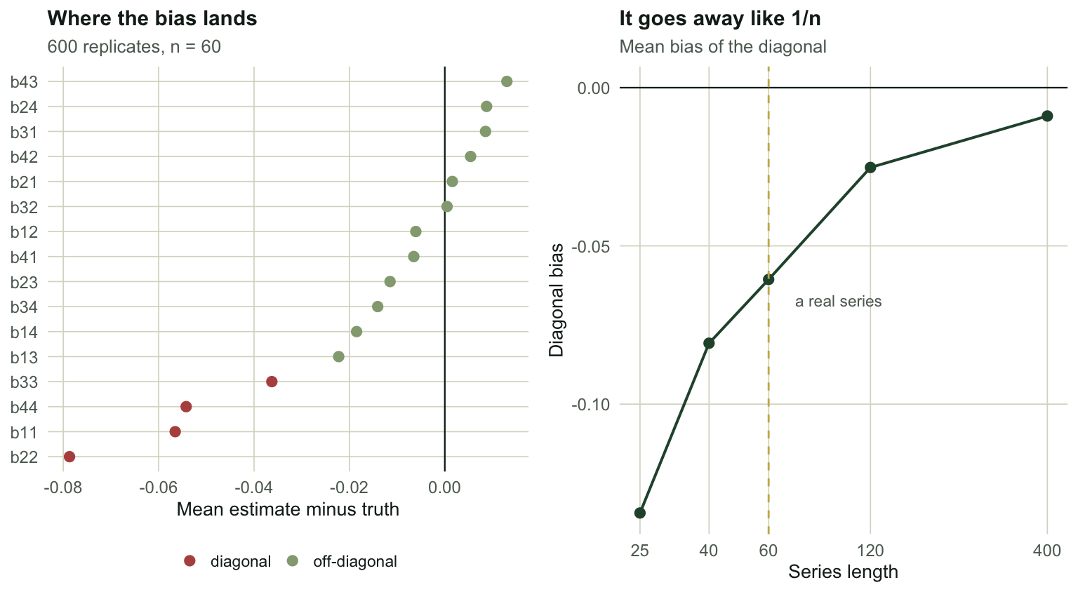
The diagonal is biased by `r sprintf("%+.4f", mean(diag(bias)))`. The off-diagonal cells average `r sprintf("%+.4f", mean(bias[row(bias) != col(bias)]))`, but that average lets cells of opposite sign cancel: their mean absolute bias is `r sprintf("%.4f", mean(abs(bias[row(bias) != col(bias)])))`, about `r sprintf("%.0f", abs(mean(diag(bias))) / mean(abs(bias[row(bias) != col(bias)])))` times smaller than the diagonal's, and in these replicates the average estimate of `r sum((sign(Btrue) * bias)[row(bias) != col(bias) & Btrue != 0] > 0)` of the `r sum(row(bias) != col(bias) & Btrue != 0)` true links sits slightly further from zero than the truth.
Read that in ecological units. The estimated diagonal is systematically too low, and a low $b_{ii}$ means fast return to the mean. **Density dependence looks stronger than it is, and most direct interactions look only slightly stronger than they are.** This is the small-sample bias of an autoregressive coefficient, known since Marriott and Pope (1954), and here it lands mainly on the diagonal, where the lagged self-terms sit. The asymmetry is a property of this parameter set rather than a law: in the shared environment below, part of the bias moves off the diagonal.
It is an $O(1/n)$ effect, so it disappears with length. Watch how slowly.
```{r}
#| label: sweep
sweep <- do.call(rbind, lapply(c(25, 40, 60, 120, 400), function(n) {
  r <- mc(n, Strue, 250, n * 1000)
  s <- apply(r$sig, c(2, 3), mean)
  z0 <- which(Btrue == 0)
  data.frame(n = n,
             bias  = mean(diag(apply(r$B, c(2, 3), mean) - Btrue)),
             mc_sd = mean(apply(r$B, c(2, 3), sd)),
             false_pos = mean(s[z0]),
             detection = mean(s[-z0]))
}))
round(sweep, 4)
```
```{r}
#| label: fig-bias
#| fig-width: 8
#| fig-height: 4.4
#| fig-cap: "Left: mean estimation error for each of the sixteen cells at n = 60, split by position. Every diagonal cell sits below zero; the off-diagonal cells straddle it. Right: the diagonal bias shrinks with series length, but sixty points still leaves close to half of it."
#| fig-alt: "Two panels. Left, a dot plot of estimation error per matrix cell showing all four diagonal cells clearly below zero and twelve off-diagonal cells scattered around zero. Right, a line showing diagonal bias rising towards zero as series length increases from twenty-five to four hundred."
cells <- data.frame(
  err  = as.vector(bias),
  kind = ifelse(as.vector(diag(4)) == 1, "diagonal", "off-diagonal"),
  cell = paste0("b", as.vector(row(bias)), as.vector(col(bias)))
)

p1 <- ggplot(cells, aes(err, reorder(cell, err), colour = kind)) +
  geom_vline(xintercept = 0, colour = te_ink, linewidth = 0.4) +
  geom_point(size = 2.2) +
  scale_colour_manual(values = c(diagonal = te_rust, `off-diagonal` = te_sage)) +
  labs(title = "Where the bias lands", subtitle = "600 replicates, n = 60",
       x = "Mean estimate minus truth", y = NULL, colour = NULL) +
  theme_te(11)

p2 <- ggplot(sweep, aes(n, bias)) +
  geom_hline(yintercept = 0, colour = te_ink, linewidth = 0.4) +
  geom_line(colour = te_forest, linewidth = 0.7) +
  geom_point(colour = te_forest, size = 2.2) +
  geom_vline(xintercept = 60, colour = te_gold, linetype = 2, linewidth = 0.5) +
  annotate("text", x = 72, y = min(sweep$bias) / 2, label = "a real series",
           hjust = 0, size = 3, colour = te_muted) +
  scale_x_log10(breaks = sweep$n, labels = sweep$n) +
  labs(title = "It goes away like 1/n", subtitle = "Mean bias of the diagonal",
       x = "Series length", y = "Diagonal bias") +
  theme_te(11)

two_panel(p1, p2)
```
At `r sweep$n[1]` points the diagonal is off by `r sprintf("%.4f", sweep$bias[1])`, which is a quarter of a typical coefficient. At `r sweep$n[5]` it is `r sprintf("%.4f", sweep$bias[5])` and gone. Sixty points, a respectable monitoring series, still carries `r sprintf("%.4f", sweep$bias[3])`.
## The screen is calibrated, and that is not enough
This community has six true zeros. Screen every cell at two standard errors and count how often a zero cell fires.
```{r}
#| label: rates
sg <- apply(r60$sig, c(2, 3), mean)
z0 <- which(Btrue == 0)
c(false_positive_on_6_true_zeros = mean(sg[z0]),
  detection_on_10_true_effects   = mean(sg[-z0]))
```
`r sprintf("%.3f", mean(sg[z0]))` on the true zeros. The screen is calibrated: it is doing about what a five per cent test should do, and nothing is broken.
Now multiply. Six zero cells at `r sprintf("%.3f", mean(sg[z0]))` is `r sprintf("%.2f", 6 * mean(sg[z0]))` false interactions per fitted model, on average. A ten-species community has ninety off-diagonal cells; if all of them were true zeros, a single honest, correctly calibrated analysis would still hand you around `r sprintf("%.0f", 90 * mean(sg[z0]))` interactions that do not exist. They will not be flagged. They will look exactly like the real ones, and the web you draw will carry them as arrows.
This is the multiple testing problem wearing an ecological hat, and the fix is the usual one: control the false discovery rate across the matrix rather than testing each cell as if it were the only cell. [The false discovery rate and Benjamini-Hochberg](../false-discovery-rate-benjamini-hochberg/) has the mechanics.
## Weak links are hard to see
Detection is not uniform across the real effects. Compare the weakest true link with a moderate one.
```{r}
#| label: weak
rbind(
  `b[1,2] = -0.10` = c(sign_error = mean(r60$B[, 1, 2] > 0), detected = sg[1, 2]),
  `b[1,3] = -0.35` = c(sign_error = mean(r60$B[, 1, 3] > 0), detected = sg[1, 3])
)
```
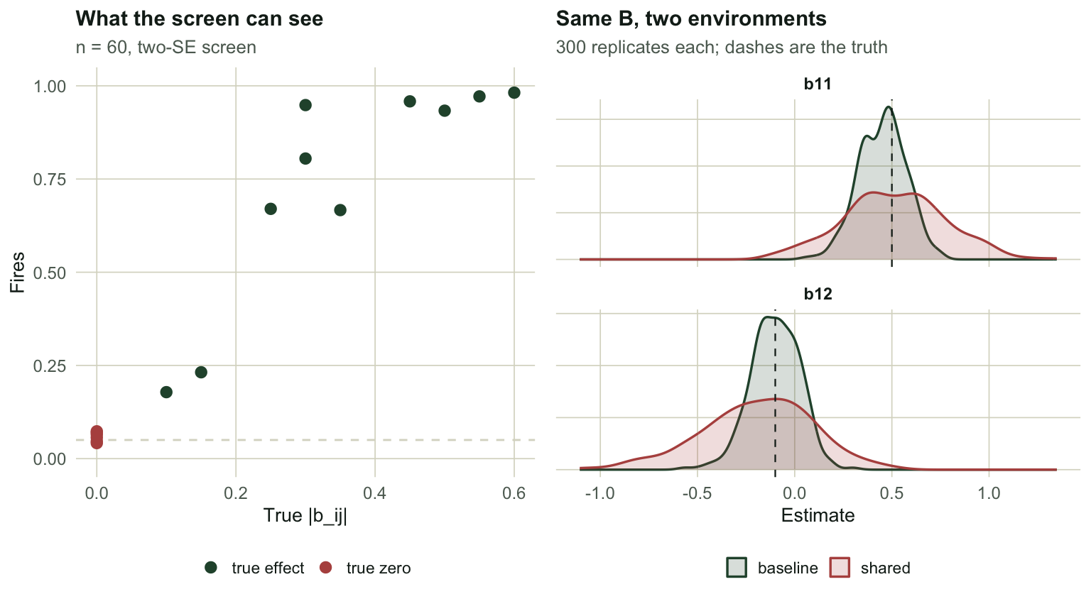
The weak competitor at $b_{12} = `r sprintf("%.2f", Btrue[1,2])`$ comes back with the **wrong sign** in `r sprintf("%.1f", 100 * mean(r60$B[, 1, 2] > 0))` per cent of replicates, and is detected in `r sprintf("%.1f", 100 * sg[1, 2])` per cent. One run in five returns a positive estimate that, read at face value, makes this competitor look like a mutualist, although almost none of those wrong-signed estimates pass the two-SE screen. The moderate link at $b_{13} = `r sprintf("%.2f", Btrue[1,3])`$ flips sign only `r sprintf("%.1f", 100 * mean(r60$B[, 1, 3] > 0))` per cent of the time.
Certain, Barraquand and Gardmark (2018) reach the same conclusion from the other direction: signs and ranks of MAR(1) coefficients survive a lot of abuse, values do not. A sixty-point series supports "species 3 suppresses species 1" and does not support "the effect is minus zero point three five".
```{r}
#| label: fig-detect
#| fig-width: 8
#| fig-height: 4.4
#| fig-cap: "Left: detection rate against the true absolute coefficient. Below about 0.2 the screen is close to blind. Right: the sampling distribution of two coefficients under the baseline environment and under a shared one, with the same true B in both."
#| fig-alt: "Two panels. Left, detection rate rising with true absolute coefficient size, with the six true zeros clustered near the origin at a low rate. Right, two overlaid density curves per coefficient showing a much wider spread when the environment is shared."
det <- data.frame(
  abs_b  = as.vector(abs(Btrue)),
  detect = as.vector(sg),
  kind   = ifelse(as.vector(Btrue) == 0, "true zero", "true effect")
)

p1 <- ggplot(det, aes(abs_b, detect, colour = kind)) +
  geom_hline(yintercept = 0.05, colour = te_line, linetype = 2, linewidth = 0.5) +
  geom_point(size = 2.4) +
  scale_colour_manual(values = c(`true effect` = te_forest, `true zero` = te_rust)) +
  ylim(0, 1) +
  labs(title = "What the screen can see", subtitle = "n = 60, two-SE screen",
       x = "True |b_ij|", y = "Detection rate", colour = NULL) +
  theme_te(11)

sdo <- function(S, seed0) {
  Bh <- array(0, c(300, p, p))
  for (m in 1:300) Bh[m, , ] <- mar1_cls(sim_mar1(60, Atrue, Btrue, S, seed = seed0 + m))$B
  Bh
}
Bb <- sdo(Strue, 11000); Bc <- sdo(Scol, 22000)

dens <- rbind(
  data.frame(v = Bb[, 1, 1], cell = "b11", env = "baseline"),
  data.frame(v = Bc[, 1, 1], cell = "b11", env = "shared"),
  data.frame(v = Bb[, 1, 2], cell = "b12", env = "baseline"),
  data.frame(v = Bc[, 1, 2], cell = "b12", env = "shared")
)
truth <- data.frame(cell = c("b11", "b12"), t = c(Btrue[1, 1], Btrue[1, 2]))

p2 <- ggplot(dens, aes(v, colour = env, fill = env)) +
  geom_density(alpha = 0.18, linewidth = 0.6) +
  geom_vline(data = truth, aes(xintercept = t), colour = te_ink, linetype = 2, linewidth = 0.4) +
  facet_wrap(~ cell, ncol = 1, scales = "free_y") +
  scale_colour_manual(values = c(baseline = te_forest, shared = te_rust)) +
  scale_fill_manual(values = c(baseline = te_forest, shared = te_rust)) +
  labs(title = "Same B, two environments", subtitle = "300 replicates each; dashes are the truth",
       x = "Estimate", y = NULL, colour = NULL, fill = NULL) +
  theme_te(11) +
  theme(axis.text.y = element_blank(), strip.text = element_text(colour = te_ink, face = "bold"))

two_panel(p1, p2)
```
## A shared environment inflates the variance
Now the third part, and the one that reaches furthest. Keep $B$ identical and correlate the environmental shocks of species 1 and 2 at `r sprintf("%.2f", Scol[1, 2] / Strue[1, 1])`, a deliberately extreme version of a shared weather signal, chosen so the mechanism shows through 300 replicates.
```{r}
#| label: vif
Xb <- sim_mar1(60, Atrue, Btrue, Strue, seed = 4269)
Xc <- sim_mar1(60, Atrue, Btrue, Scol,  seed = 4269)

vf <- function(M) {
  Ml <- M[-nrow(M), ]
  sapply(1:p, function(j) 1 / (1 - summary(lm(Ml[, j] ~ Ml[, -j]))$r.squared))
}
rbind(baseline = vf(Xb), shared = vf(Xc))
```
The predictors in a MAR(1) design *are* the species, so environmental synchrony is collinearity in the design matrix. The variance inflation factor for species 1 goes from `r sprintf("%.2f", vf(Xb)[1])` to `r sprintf("%.2f", vf(Xc)[1])` and for species 2 from `r sprintf("%.2f", vf(Xb)[2])` to `r sprintf("%.2f", vf(Xc)[2])`. Species 3 and 4, whose environments were left alone, barely move.
The cost lands on the coefficients that involve the synchronised pair.
```{r}
#| label: sd-inflation
sb <- apply(Bb, c(2, 3), sd); sc <- apply(Bc, c(2, 3), sd)
tab <- t(sapply(list(c(1, 1), c(1, 2), c(2, 1)), function(ij) {
  c(baseline = sb[ij[1], ij[2]], shared = sc[ij[1], ij[2]],
    ratio = sc[ij[1], ij[2]] / sb[ij[1], ij[2]])
}))
rownames(tab) <- c("b[1,1]", "b[1,2]", "b[2,1]")
round(tab, 3)
```
The sampling standard deviation of $b_{11}$ goes from `r sprintf("%.3f", sb[1,1])` to `r sprintf("%.3f", sc[1,1])`, a factor of `r sprintf("%.2f", sc[1,1]/sb[1,1])`. For $b_{12}$ it is `r sprintf("%.2f", sc[1,2]/sb[1,2])`. Nothing about the ecology changed. Two species started responding to the same weather, and the data became much less able to tell their interaction apart from their shared response: the coefficients are still identified, but their sampling spread more than doubled. The small-sample bias moves as well: across the same shared-environment replicates the mean error of $b_{11}$ is `r sprintf("%+.3f", mean(Bc[, 1, 1]) - Btrue[1, 1])` and that of the weak competitor $b_{12}$ is `r sprintf("%+.3f", mean(Bc[, 1, 2]) - Btrue[1, 2])`, so the weak competitor now looks stronger than it is while the self-term of species 1 is close to unbiased.
Which is the ordinary lesson of collinearity, arriving through a door ecologists do not usually watch. [Collinearity and VIF](../collinearity-and-vif/) is the static version of exactly this; here the correlated predictors are the community itself.
## The honest limit
Three separate things degrade a MAR(1) interaction estimate, and they do not degrade it in the same way.
The small-sample bias is systematic, sits mainly on the diagonal under the baseline shocks, and shrinks predictably with length. You can reason about it. The screening error rate is calibrated per cell and catastrophic per matrix, and the fix is a multiple-comparisons fix. Neither of those is fatal.
The third comes closer. Environmental synchrony inflates the variance of exactly the coefficients you most want, and no amount of care in the fitting recovers what the design does not contain. A long series helps; a synchronised community needs something other than the abundance series to break the tie.
So the reportable output of a sixty-point MAR(1) fit is a sign structure with a false-discovery control on it, not a table of interaction strengths to two decimal places. [Community stability from a MAR(1) model](../stability-from-a-mar1-model/) is the next question: what happens when you feed these coefficients into a stability metric.
## References
- Ives AR, Dennis B, Cottingham KL, Carpenter SR 2003 Ecological Monographs 73(2):301-330 (10.1890/0012-9615(2003)073[0301:ECSAEI]2.0.CO;2)
- Marriott FHC, Pope JA 1954 Biometrika 41(3-4):390-402 (10.1093/biomet/41.3-4.390)
- Certain G, Barraquand F, Gardmark A 2018 Methods in Ecology and Evolution 9(9):1975-1995 (10.1111/2041-210X.13021)
- Hampton SE, Holmes EE, Scheef LP, Scheuerell MD, Katz SL, Pendleton DE, Ward EJ 2013 Ecology 94(12):2663-2669 (10.1890/13-0996.1)
## Related tutorials
- [Fitting a MAR(1) model to community time series](../fitting-a-mar1-model/)
- [Community stability from a MAR(1) model](../stability-from-a-mar1-model/)
- [Checking a MAR(1) model](../checking-a-mar1-model/)
- [Aggregation and host parasitoid stability](../aggregation-and-host-parasitoid-stability/)