The S-map and state-dependent dynamics

Build the S-map in base R, test whether population dynamics are state dependent rather than linear, and see when its interaction coefficients are real and when they are noise.

Simplex projection answers a yes or no question: is there state-dependent structure that a linear model misses? The S-map answers the follow-up. It measures how much state dependence there is, on a continuous dial, and it hands you a local linear model at every point on the attractor.

That second part is what made the method popular in ecology. If the local model’s coefficients are the partial derivatives of the dynamics, then the coefficient on species j in species i’s equation is the interaction strength between them, at that moment, and it can change through time. Interaction strengths that fluctuate with the state of the community: that is a genuinely new kind of measurement, and it is also where the method is easiest to over-read.

This post builds the S-map, uses it as a nonlinearity test, and then shows the same estimator recovering one interaction coefficient and fabricating another, in the same system, from the same data, at the same settings.

From a global line to a local one

Fit a linear autoregressive model and you get one set of coefficients for the whole series. The system is assumed to behave the same way at low density as at high density. The S-map keeps the linear form but refits it for every point you want to predict, weighting the other points by how far they are from that point in state space:

\[w_i = \exp\!\left(-\theta \frac{d_i}{\bar{d}}\right)\]

where d_i is the distance from the target point to library point i, and dbar the mean of those distances. Then it solves a weighted least squares problem and uses those coefficients for that one prediction.

The dial is theta. At theta = 0 every point gets weight one, the weighting disappears, and the S-map is the global linear model. As theta grows, distant points fade out and the fit becomes local, so the effective model changes as the system moves around its attractor. Nothing else about the method changes: same form, same data, one number.

That construction is what makes the test work. Comparing theta = 0 against theta > 0 is not comparing two different models with different numbers of parameters; it is the same model at two settings of one dial. If skill improves as the fit localises, the dynamics depend on the state.

The engine

make_block <- function(x, E, tau = 1) {
  n <- length(x)
  tt <- seq((E - 1) * tau + 1, n)
  M <- matrix(NA_real_, nrow = length(tt), ncol = E)
  for (j in seq_len(E)) M[, j] <- x[tt - (j - 1) * tau]
  list(M = M, t = tt)
}

## S-map over an arbitrary state matrix M predicting target y
smap_block <- function(M, y, theta = 0, loo = TRUE) {
  n <- nrow(M)
  D <- as.matrix(dist(scale(M)))          # standardise: coordinates share a scale
  A0 <- cbind(1, M)
  cf <- matrix(NA_real_, n, ncol(M) + 1)
  pred <- rep(NA_real_, n)
  for (i in seq_len(n)) {
    use <- if (loo) seq_len(n) != i else rep(TRUE, n)
    d <- D[i, use]
    w <- exp(-theta * d / mean(d))
    A <- A0[use, , drop = FALSE] * w
    b <- y[use] * w
    sv <- svd(A)                          # SVD solve: weights make A ill-conditioned
    tol <- max(dim(A)) * .Machine$double.eps * max(sv$d)
    co <- as.numeric(sv$v %*% (ifelse(sv$d > tol, 1 / sv$d, 0) * crossprod(sv$u, b)))
    cf[i, ] <- co
    pred[i] <- sum(c(1, M[i, ]) * co)
  }
  list(coef = cf, pred = pred, rho = cor(pred, y))
}

smap <- function(x, E, tau = 1, tp = 1, theta = 0, loo = TRUE) {
  bl <- make_block(x, E, tau)
  ok <- (bl$t + tp) <= length(x)
  smap_block(bl$M[ok, , drop = FALSE], x[bl$t[ok] + tp], theta = theta, loo = loo)
}

Two details earn their place. Distances are computed on standardised coordinates, so a variable measured in thousands does not swamp one measured in units. And the weighted system is solved by SVD rather than solve, because at high theta most weights are near zero and the design matrix becomes ill conditioned; the singular value cutoff keeps that from blowing up silently.

Check the claim before using it

If theta = 0 really is the global linear model, then the S-map at that setting, run on the full library with no leave-one-out, must reproduce lm exactly. Worth checking rather than believing.

gen_ricker <- function(n, burn = 500, r = 3.0, x0 = 0.6) {
  N <- n + burn; x <- numeric(N); x[1] <- x0
  for (t in 1:(N - 1)) x[t + 1] <- x[t] * exp(r * (1 - x[t]))
  x[(burn + 1):N]
}

set.seed(4265)
n <- 300
z <- gen_ricker(n) * exp(rnorm(n, 0, 0.05))    # 5% observation error

s0 <- smap(z, E = 2, tp = 1, theta = 0, loo = FALSE)
X <- embed(z, 3)
m_lm <- lm(X[, 1] ~ X[, 2] + X[, 3])
coef_gap <- max(abs(sweep(s0$coef, 2, coef(m_lm))))
fit_gap <- max(abs(s0$pred - fitted(m_lm)))

The largest disagreement between the S-map’s coefficients and lm’s is 3.6e-15, and between the fitted values 2.1e-14. Machine epsilon. The S-map at theta = 0 is not like a linear autoregressive model, it is one.

The nonlinearity test

Now turn the dial. The chaotic Ricker series from the previous post, and its linear counterpart: an autoregressive model fitted to it and simulated from, so the two share their autocorrelation structure and differ only in whether a deterministic map is underneath.

ar_fit <- ar(z, order.max = 10, method = "mle")
set.seed(9265)
z_lin <- as.numeric(arima.sim(n = n, model = list(ar = ar_fit$ar),
                              sd = sqrt(ar_fit$var.pred)))

thetas <- c(0, 0.1, 0.3, 0.5, 1, 2, 3, 4, 6, 8)
rho_chaos <- sapply(thetas, function(th) smap(z, E = 2, tp = 1, theta = th)$rho)
rho_lin <- sapply(thetas, function(th) smap(z_lin, E = 2, tp = 1, theta = th)$rho)

gain_chaos <- max(rho_chaos) - rho_chaos[1]
gain_lin <- max(rho_lin) - rho_lin[1]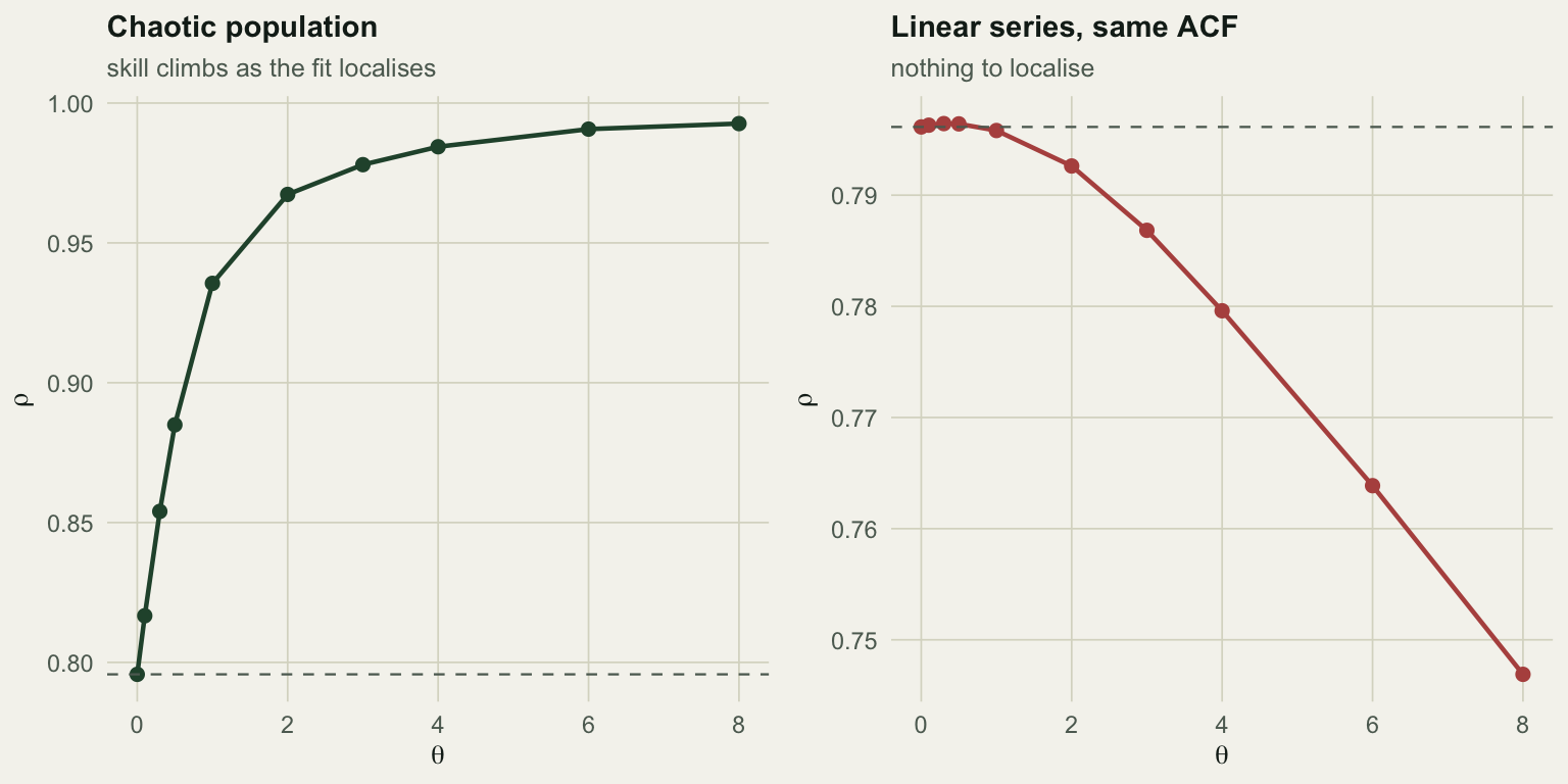

Figure 1: Forecast skill against the S-map localisation parameter. The chaotic series improves steeply as the fit becomes local; the linear series with matching autocorrelation gains nothing and then degrades.

The chaotic series goes from rho = 0.796 at theta = 0 to 0.993 at its best, a gain of +0.197. The linear series starts at 0.796 and its best is 0.796, a gain of +0.000, which is nothing. Push theta further and the linear series gets actively worse (0.747 at theta = 8), because localising a fit that has no local structure to find just throws away data.

This is the cleanest test in the toolkit. Same model, same data, one dial, and the answer is a comparison against a value the method itself produces at theta = 0. A dashed line marks that baseline in both panels.

Interaction coefficients that move

The dial test uses one species. The coefficients need more. If you have measured several species, use their contemporaneous values as the state instead of lagged values of one, and predict one species forward. The local coefficients are then estimates of

\[\frac{\partial\, x_{i,t+1}}{\partial\, x_{j,t}}\]

at each point in time: how much species j currently affects species i.

The test system is two competitors with asymmetric coupling, and we know its Jacobian exactly. Species X drives Y with strength 0.10; Y drives X with strength 0.02. Both are chaotic, and their abundances are almost uncorrelated.

gen_coupled <- function(n, burn = 500, rx = 3.8, ry = 3.5,
                        bxy = 0.02, byx = 0.1, x0 = 0.4, y0 = 0.2) {
  N <- n + burn; x <- numeric(N); y <- numeric(N); x[1] <- x0; y[1] <- y0
  for (t in 1:(N - 1)) {
    x[t + 1] <- x[t] * (rx - rx * x[t] - bxy * y[t])
    y[t + 1] <- y[t] * (ry - ry * y[t] - byx * x[t])
  }
  data.frame(x = x[(burn + 1):N], y = y[(burn + 1):N])
}

set.seed(4265)
nc <- 400
d <- gen_coupled(nc)
M <- cbind(x = d$x[-nc], y = d$y[-nc])

## true Jacobian entries, from differentiating the model by hand
true_YX <- -0.10 * M[, "y"]                          # d y[t+1] / d x[t] : strong link
true_XY <- -0.02 * M[, "x"]                          # d x[t+1] / d y[t] : weak link
true_XX <- 3.8 - 2 * 3.8 * M[, "x"] - 0.02 * M[, "y"]

th_grid <- c(0, 0.5, 1, 2, 3, 4, 6, 8)
rho_X <- sapply(th_grid, function(th) smap_block(M, d$x[-1], theta = th)$rho)
rho_Y <- sapply(th_grid, function(th) smap_block(M, d$y[-1], theta = th)$rho)
th_best <- th_grid[which.max(rho_Y)]

fitX <- smap_block(M, d$x[-1], theta = th_best)      # x[t+1] ~ (x[t], y[t])
fitY <- smap_block(M, d$y[-1], theta = th_best)      # y[t+1] ~ (x[t], y[t])

est_YX <- fitY$coef[, 2]     # coefficient on x in the y equation : strong link
est_XY <- fitX$coef[, 3]     # coefficient on y in the x equation : weak link
est_XX <- fitX$coef[, 2]     # self effect : strong

cor_strong <- cor(est_YX, true_YX)
cor_weak <- cor(est_XY, true_XY)
cor_self <- cor(est_XX, true_XX)

Cross validation picks theta = 8 and the forecasts are near perfect (rho = 1.0000 for the Y equation). Now compare each estimated coefficient against the truth we can compute analytically.

Figure 2: Estimated S-map interaction coefficients against the true Jacobian entries, for the strong link and the weak link in the same system at the same settings.

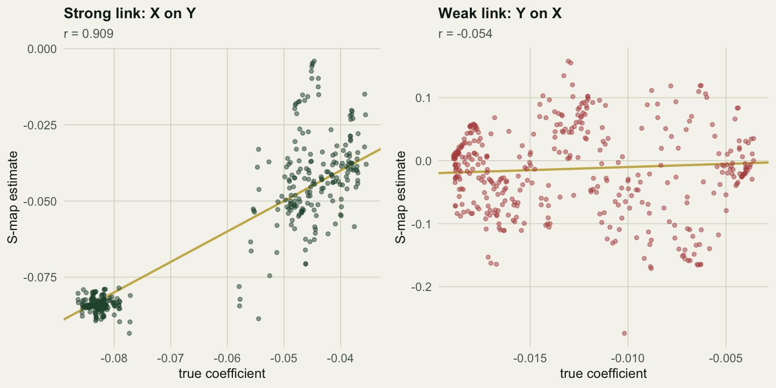
The strong link is recovered: the estimated coefficients track the true ones at a correlation of 0.909, and their mean, -0.0631, sits on the true mean of -0.0637. The self effect comes back too, at 0.997. Given that the two species’ abundances correlate at only 0.11, recovering a time-varying interaction this well from the raw series is a real result.

The weak link is not recovered. The estimates correlate with the truth at -0.054: no relationship at all.

The part to be careful about

Look at the right panel again. Those estimates are not flat, not obviously broken, and not implausible. Their mean is -0.0160 against a true mean of -0.0127, which is close enough to pass a sanity check. Plot them against time and you get a wiggly line that looks exactly like a fluctuating interaction strength. Every diagnostic available within the analysis is green: the forecasts are near perfect, theta was chosen by cross validation, the self terms and the strong cross term validate beautifully against the truth in the same fit.

And the time course is noise.

The reason is simple once stated. The weak coefficient is about 5 times smaller than the strong one and roughly two orders of magnitude smaller than the self term, which ranges over several units. A local linear fit has to separate that contribution from everything else happening in a neighbourhood of the attractor, and it cannot. Nothing warns you, because the quantity that fails is not the one the diagnostics measure: prediction is dominated by the large terms, so the model predicts brilliantly while the small coefficient it reports is arbitrary.

This is the honest limit of S-map interaction strengths, and it is not an artefact of a hard example. It is the ordinary case in community ecology, where most pairwise effects are weak and a few are strong. The practical reading:

• The average of a coefficient can be informative even when its fluctuations are not. Here the weak link’s mean was roughly right while its time course was noise. Reporting “the interaction varied through time from A to B” is a much stronger claim than reporting its average, and it needs much more support.
• The coefficients you can trust are the ones large enough to drive the prediction, which is circular but real: strength and identifiability are the same axis.
• Validate on something. A simulation with a known Jacobian, a perturbation experiment, an independent estimate of the interaction. If nothing anchors the coefficient, its wiggles are decoration.
• At theta = 0 the coefficients are useless even for the strong link, because a single global line through a curved map has no local derivative to report. Localisation is what makes the coefficients mean anything, and it is also what makes them variable.

There is a further wrinkle worth knowing about: with several species the local design matrix is often close to collinear, and the coefficient split between correlated species is then poorly determined even when their sum is not. Regularised versions of the S-map exist for exactly this reason (Cenci and colleagues), and the reason they exist is that the plain version is fragile.

Where to go next

Two of these coefficients said the same thing about the true structure, in opposite directions: X affects Y appreciably, Y affects X hardly at all. The S-map got the strong one right and the weak one wrong, but it needed both species measured to say anything at all.

The next question is what to do when you cannot measure both, or when you can but want to know which one is driving which. Convergent cross mapping attacks that directly, and it needs only the reconstruction from the previous post. It also inherits every fragility on display here, plus some of its own, which is what the checking post is for.

References

Ushio, Hsieh, Masuda, Deyle, Ye, Chang, Sugihara & Kondoh 2018 Nature 554(7692):360-363 (10.1038/nature25504)

Sugihara 1994 Philosophical Transactions of the Royal Society A 348(1688):477-495 (10.1098/rsta.1994.0106)

Deyle, May, Munch & Sugihara 2016 Proceedings of the Royal Society B 283(1822):20152258 (10.1098/rspb.2015.2258)

Cenci, Sugihara & Saavedra 2019 Methods in Ecology and Evolution 10(5):650-660 (10.1111/2041-210X.13150)

Hsieh, Glaser, Lucas & Sugihara 2005 Nature 435(7040):336-340 (10.1038/nature03553)

Sugihara, May, Ye, Hsieh, Deyle, Fogarty & Munch 2012 Science 338(6106):496-500 (10.1126/science.1227079)

Related tutorials

• Simplex projection and delay embedding
• Convergent cross mapping in ecology
• Checking an empirical dynamic model
• Checking a penalised regression