make_block <- function(x, E, tau = 1) {
  n <- length(x)
  tt <- seq((E - 1) * tau + 1, n)
  M <- matrix(NA_real_, nrow = length(tt), ncol = E)
  for (j in seq_len(E)) M[, j] <- x[tt - (j - 1) * tau]
  list(M = M, t = tt)
}

simplex <- function(x, E, tau = 1, tp = 1, theiler = 0, target = NULL) {
  if (is.null(target)) target <- x
  bl <- make_block(x, E, tau)
  M <- bl$M; tt <- bl$t
  ok <- (tt + tp) >= 1 & (tt + tp) <= length(target)
  M <- M[ok, , drop = FALSE]; tt <- tt[ok]
  y <- target[tt + tp]
  D <- as.matrix(dist(M))
  pred <- rep(NA_real_, length(tt))
  for (i in seq_along(tt)) {
    d <- D[i, ]
    d[abs(tt - tt[i]) <= theiler] <- Inf   # drop self and temporal neighbours
    o <- order(d)[seq_len(E + 1)]
    dn <- d[o]
    if (!all(is.finite(dn))) next
    w <- if (dn[1] == 0) as.numeric(dn == 0) else exp(-dn / dn[1])
    w <- pmax(w, 1e-8)
    pred[i] <- sum(w * y[o]) / sum(w)
  }
  keep <- !is.na(pred)
  list(rho = suppressWarnings(cor(pred[keep], y[keep])),
       pred = pred, obs = y, t = tt)
}Simplex projection and delay embedding
R
EDM
time series
nonlinear dynamics
ecology tutorial
Reconstruct a population’s attractor from one time series, forecast it with simplex projection in base R, and separate deterministic dynamics from linear noise.
Corrected 8 October 2026: the post said that scoring simplex leave-one-out against an in-sample linear model is what keeps the gain negative on the linear replicates, so that the comparison leans against a false positive by construction; that handicap is small and choosing the best embedding dimension favours simplex, so the text now credits the nearest-neighbour forecast losing on a linear series. It also said the comparison series has the same second-order structure as the original, where it only closely matches it, and that the S-map tests which variables make up the state, where it measures state dependence.
Corrected 1 October 2026: the summary said the method separates deterministic dynamics from red noise, but the linear comparison series is negatively autocorrelated, the opposite of red noise; it now calls that series linear noise.
Corrected 27 September 2026: the caption and alt text of the forecast-horizon figure said both methods had fallen to about zero at eight steps on the linear series; as drawn, both are weak there (about 0.1 to 0.2) and simplex ends slightly above the linear model.
An annual count series wobbles up and down for thirty years. The autocorrelation function says the wobble is not white noise, and an ARIMA model fits it well enough. Nothing in that workflow can tell you whether the wobble comes from a low-dimensional deterministic system that you could, in principle, forecast, or from a linear process pushed around by weather.
Empirical dynamic modelling asks the question the other way round. Instead of fitting an equation, it treats the series as a shadow of a trajectory moving on an attractor, and reconstructs that attractor from the series itself. This post builds the two pieces you need: the delay embedding, and simplex projection, the nearest-neighbour forecast that runs on it. Both are twenty lines of base R.
The payoff is a test that no linear model can perform: does knowing where the system is now, in reconstructed state space, tell you more about the next step than the best linear predictor can? For the series below the answer is yes, and the same machinery says no for a linear series with a closely matching autocorrelation function.
The idea: one variable carries the whole attractor
A population does not live in one dimension. Abundance next year depends on abundance now, on the predator, on the nutrient pool, on whatever else is coupled to it. That full state is a point moving on an attractor in some multi-dimensional space, and you measured one coordinate of it.
Takens showed that this is enough. Under mild conditions, the vector of lagged values
\[\mathbf{v}_t = \big(x_t,\; x_{t-\tau},\; x_{t-2\tau},\; \ldots,\; x_{t-(E-1)\tau}\big)\]
traces out a shape that is a faithful copy of the true attractor: distinct states stay distinct, and nearby points stay nearby. The unmeasured variables leave their fingerprint in the history of the one you did measure. E is the embedding dimension and tau the lag; for annual ecological series tau = 1 is almost always the right choice, so the only real knob is E.
The practical consequence is the one that matters here. If the reconstruction is faithful, then points that are close in delay coordinates are close in the true state, so they should do the same thing next. That turns forecasting into a lookup: find the neighbours, see where they went, average.
The engine
Two functions. make_block stacks the delay vectors; simplex finds the E+1 nearest neighbours of each point, weights them by distance, and predicts tp steps ahead. The prediction for each point leaves that point out, so nothing is fitted to itself.
The weights exp(-d / d1) scale each neighbour by its distance relative to the closest one, so an identical past state dominates and a far-off state barely contributes. The simplex of E+1 points is the smallest set that can enclose a point in E dimensions, which is where the method gets its name.
theiler deserves a note now and a warning later. Setting it to zero drops only the point being predicted. Setting it higher drops every library point within that many time steps, which is how you stop the method from “forecasting” a point by interpolating between its immediate neighbours in time.
A population that is deterministic and unpredictable
The Ricker map is the standard single-species chaotic population model: density dependence with overcompensation, no external forcing, no process noise. At an intrinsic growth rate of 3.0 it is chaotic. Every value follows exactly from the one before, and yet the series looks like noise.
We measure it with 10 per cent lognormal observation error, which is optimistic for a real count survey and still enough to matter.
gen_ricker <- function(n, burn = 500, r = 3.0, x0 = 0.6) {
  N <- n + burn; x <- numeric(N); x[1] <- x0
  for (t in 1:(N - 1)) x[t + 1] <- x[t] * exp(r * (1 - x[t]))
  x[(burn + 1):N]
}

set.seed(4264)
n <- 300
z_true <- gen_ricker(n)
z <- z_true * exp(rnorm(n, 0, 0.10))     # 10% observation error

acf1 <- acf(z, plot = FALSE)$acf[2]
The lag-1 autocorrelation is -0.71. The comparison series is the honest linear counterpart: fit an autoregressive model to the chaotic series, then simulate from it. By construction its second-order structure closely matches the original’s, and it has no determinism whatsoever.
ar_fit <- ar(z, order.max = 10, method = "mle")
set.seed(9264)
z_lin <- as.numeric(arima.sim(n = n, model = list(ar = ar_fit$ar),
                              sd = sqrt(ar_fit$var.pred)))
acf1_lin <- acf(z_lin, plot = FALSE)$acf[2]
An AR(6) was selected, and the simulated series has lag-1 autocorrelation -0.75 against the original’s -0.71. To the autocorrelation function these two series are near twins.
The picture that gives the game away
Plot each value against the one before it. This is the two-dimensional delay embedding, and for a one-dimensional map it is the map.
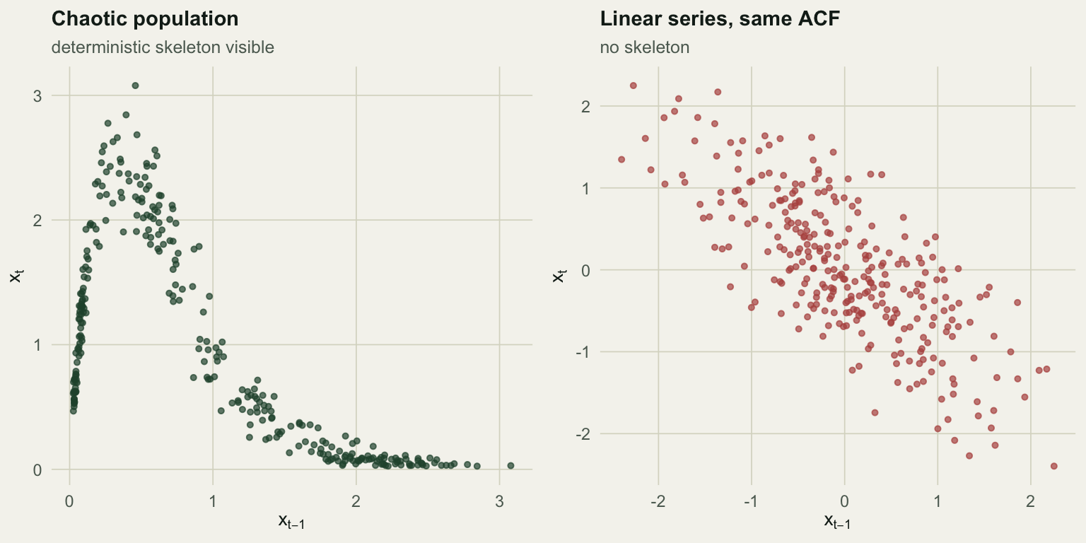
Both series have effectively the same lag-1 autocorrelation. One of them is a curve with a little observation scatter around it, the other is a cloud. Every summary that stops at second-order structure treats them as equivalent; the lag plot does not, and neither does simplex projection.
For a real system with more than one dimension the picture is not this generous, which is exactly why the forecast skill, not the eyeball, has to do the work.
Choosing the embedding dimension
Run simplex at E = 1 to 8 and keep the E that forecasts best. For a one-dimensional map like the Ricker the true answer is E = 1.
Es <- 1:8
rho_E <- sapply(Es, function(E) simplex(z, E = E, tp = 1)$rho)
rho_E_lin <- sapply(Es, function(E) simplex(z_lin, E = E, tp = 1)$rho)
E_best <- Es[which.max(rho_E)]
E_best_lin <- Es[which.max(rho_E_lin)]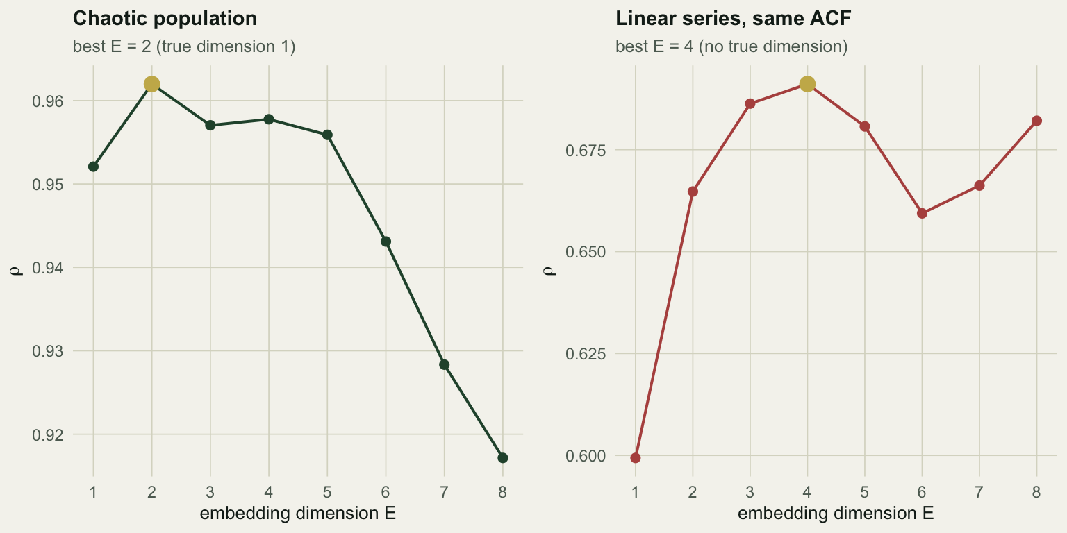
The chaotic series peaks at E = 2 with rho = 0.962, but the curve barely moves: across E = 1 to 4 the skill spans only 0.010, so the position of that peak is a weak guide to the true dimension of one. The linear series peaks at E = 4, and that number means nothing at all either: the series has no attractor and no dimension. A peak in this curve is not evidence of determinism, it is just the point where the bias and variance of a nearest-neighbour average happen to balance. The peak location is the first thing people over-read in EDM, and the first honest limit of this post.
The test: does the nonlinear forecast beat the linear one?
The comparison that carries information is not simplex against nothing, it is simplex against the best linear model you can build from the same data. If a linear autoregressive model does as well, the reconstruction has bought you nothing.
We give the linear model an advantage on purpose. Its coefficients are fitted on the whole series and it predicts in sample, while simplex leaves each point out. If simplex still wins, the result is not an artefact of a generous comparison.
lin_rho <- function(x, p, tp) {
  n <- length(x)
  X <- embed(x, p + 1)
  cf <- coef(lm(X[, 1] ~ X[, -1, drop = FALSE]))
  pr <- rep(NA_real_, n)
  for (t in p:(n - tp)) {
    st <- x[t:(t - p + 1)]
    for (k in 1:tp) {                       # iterate the linear map forward
      nx <- cf[1] + sum(cf[-1] * st)
      st <- c(nx, st[-p])
    }
    pr[t + tp] <- st[1]
  }
  ok <- !is.na(pr)
  cor(pr[ok], x[ok])
}

tps <- 1:8
sx_chaos <- sapply(tps, function(tp) simplex(z, E = E_best, tp = tp)$rho)
ln_chaos <- sapply(tps, function(tp) lin_rho(z, ar_fit$order, tp))

ar_lin <- ar(z_lin, order.max = 10, method = "mle")
sx_lin <- sapply(tps, function(tp) simplex(z_lin, E = E_best_lin, tp = tp)$rho)
ln_lin <- sapply(tps, function(tp) lin_rho(z_lin, ar_lin$order, tp))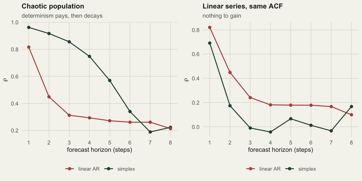
On the chaotic series simplex reaches rho = 0.962 one step ahead against the linear model’s 0.816, and the gap widens at two steps (0.917 against 0.449). On the linear series the ordering flips: simplex gets 0.691 and the linear model 0.820. The nonlinear machinery loses, as it should, because there is nothing nonlinear to find.
Two separate things are visible in the chaotic panel. The gap between the curves is the determinism: state-space structure that a linear model cannot represent. The decline of the simplex curve, from 0.962 at one step to 0.223 at eight, is chaos itself: nearby trajectories separate exponentially, so knowing the state now buys less and less about the state later. A deterministic system can be perfectly knowable and still unforecastable beyond a few steps. That decay rate is a rough read on the Lyapunov exponent, and it is the thing that makes “deterministic” and “predictable” different words.
How reliable is the verdict?
The gap is a difference of two correlations, not a test statistic. It has no null distribution attached, so the sensible question is how often it points the wrong way. Sixty replicate series of the linear process, and thirty of the chaotic one:
gain <- function(x, Emax = 6) {
  rr <- sapply(1:Emax, function(E) simplex(x, E = E, tp = 1)$rho)
  p <- max(1, ar(x, order.max = 6, method = "mle")$order)
  X <- embed(x, p + 1)
  max(rr) - cor(fitted(lm(X[, 1] ~ X[, -1, drop = FALSE])), X[, 1])
}

set.seed(3264)
g_null <- replicate(60, gain(as.numeric(arima.sim(n = 200, model = list(ar = ar_fit$ar),
                                                  sd = sqrt(ar_fit$var.pred)))))
g_chaos <- replicate(30, gain(gen_ricker(200, x0 = runif(1, 0.3, 0.9)) *
                              exp(rnorm(200, 0, 0.10))))
fp <- mean(g_null > 0)
tp_rate <- mean(g_chaos > 0)
The gain is positive in 0% of the linear replicates and 100% of the chaotic ones. The direction is trustworthy here, but the design is not what produces it. Simplex is handicapped by leave-one-out while the linear model is not, yet simplex also keeps the best of several embedding dimensions, so the comparison does not lean against a false positive by construction. The linear replicates stay negative because, with nothing nonlinear to find, a nearest-neighbour forecast does worse than the linear model, as it did on the single linear series above. That is an empirical result for this process and these series lengths, not a calibrated size. If you want a p-value, you need a null that preserves the linear structure and destroys the determinism, which is what the phase-randomised surrogate does, and what the checking post uses.
Where this breaks
The best E moves with the noise. Repeat the sweep at three observation-error levels:
set.seed(5264)
noise_levels <- c(0, 0.05, 0.10, 0.20)
E_by_noise <- sapply(noise_levels, function(s) {
  zz <- z_true * exp(rnorm(n, 0, s))
  which.max(sapply(1:8, function(E) simplex(zz, E = E, tp = 1)$rho))
})
rho_flat <- diff(range(rho_E[1:4]))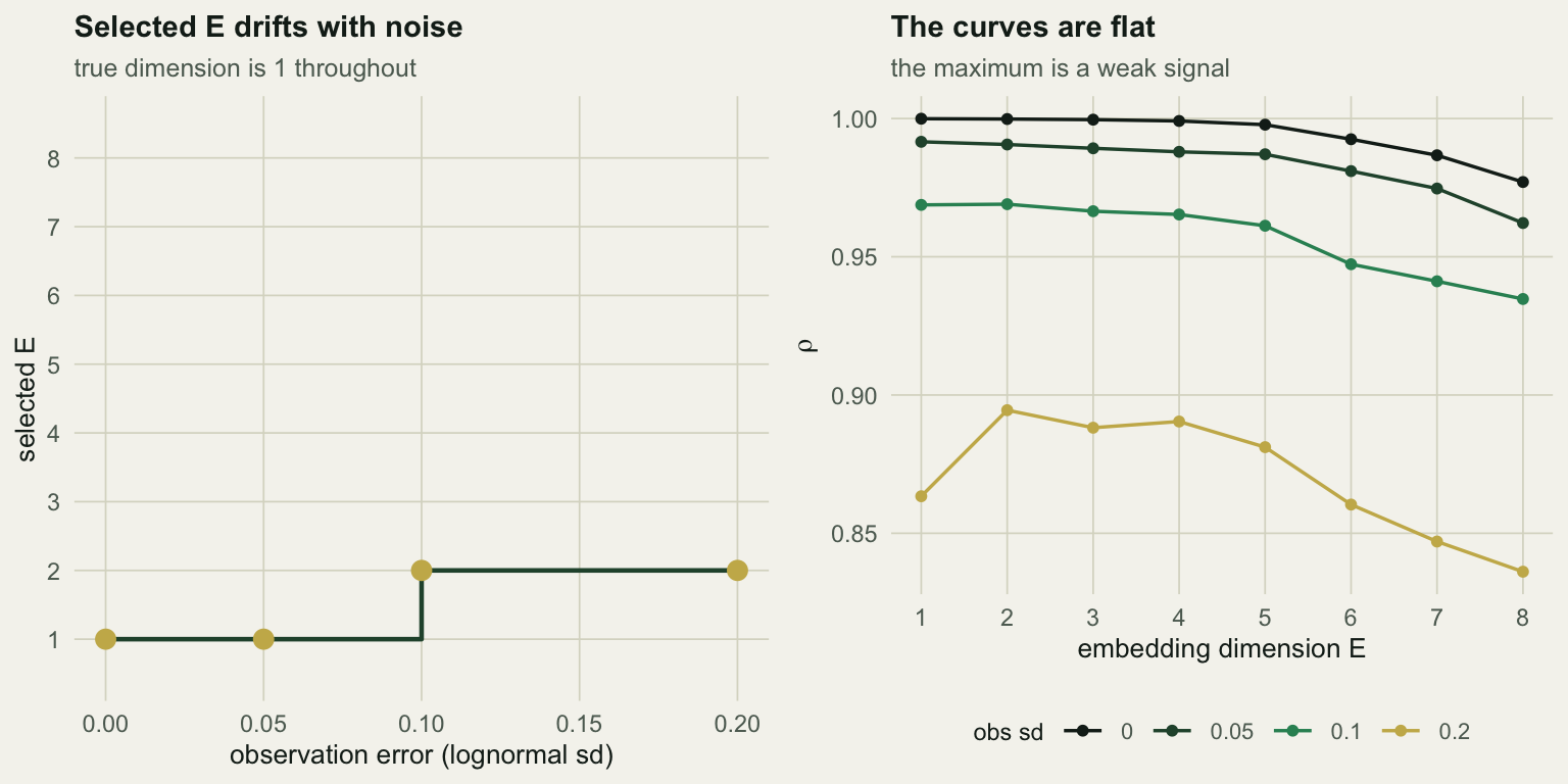
With no observation error the sweep returns E = 1, the truth. Add error and the choice drifts to 1, 2, 2 at 5, 10, 20 per cent. The true dimension never changed.
Look closely at the 10 per cent case and see how little the choice rests on. The main analysis above, on a series with exactly that much error, selected E = 2; this sweep, at the same error level but a different random draw, selects E = 2, against a true dimension of one in both cases. Across E = 1 to 4 the skill on the original series spans only 0.010, which is the most that the winning E can be ahead of any of its neighbours in that range. All four series in the sweep carry the same deterministic skeleton and differ only in the observation error laid over it, so a maximum picked out of a band that narrow is reporting the noise as much as the dynamics. Report the curve, not just its maximum, and check that your conclusions survive the neighbouring values of E.
Temporal neighbours are not state-space neighbours. With a smooth, densely sampled series the closest point in delay space is often the one immediately before or after in time. Predicting from those is interpolation dressed up as forecasting, and the skill it reports is not out-of-sample in any useful sense. The theiler argument exists for this; set it to something like the decorrelation time and see whether the skill survives. It matters most for high-frequency data (loggers, camera traps, daily counts) and least for annual series, where consecutive years are already far apart on the attractor.
Determinism is not the same as low dimension, and neither is the same as knowing the mechanism. A good simplex forecast says the system has state-dependent structure that a linear model misses. It does not say which variables make up the state, whether the dynamics are stationary, or what causes what. The S-map turns the state dependence itself into a quantitative test, and convergent cross mapping takes on what causes what.
Where to go next
The reconstruction is the foundation for everything else in this cluster. Once you trust that M_x is a faithful copy of the attractor, two things follow. First, the local structure can be turned into a smoothly tunable model that measures how nonlinear the dynamics are, which is the S-map. Second, if two species are dynamically coupled, each one’s reconstruction carries the other’s signature, which is what makes causal inference from time series possible at all.
Before applying any of it to a real series, be clear about what you have. Thirty annual counts are not going to reconstruct anything: the library is too small for nearest neighbours to be near. The methods here need hundreds of points, or a great deal of luck.
References
Takens 1981 Lecture Notes in Mathematics 898:366-381 (10.1007/BFb0091924)
Sugihara, May 1990 Nature 344(6268):734-741 (10.1038/344734a0)
Sugihara, May, Ye, Hsieh, Deyle, Fogarty, Munch 2012 Science 338(6106):496-500 (10.1126/science.1227079)
Hsieh, Glaser, Lucas, Sugihara 2005 Nature 435(7040):336-340 (10.1038/nature03553)
Deyle, Sugihara 2011 PLoS ONE 6(3):e18295 (10.1371/journal.pone.0018295)
Chang, Ushio, Hsieh 2017 Ecological Research 32(6):785-796 (10.1007/s11284-017-1469-9)
Theiler 1986 Physical Review A 34(3):2427-2432 (10.1103/PhysRevA.34.2427)