Convergent cross mapping in ecology

Detect which species drives which from time series alone. Build CCM in base R, read the direction correctly, and learn why convergence, not a high correlation, is the test.

Two species fluctuate for four hundred generations. One drives the other five times harder than it is driven back. Their abundances correlate at 0.11.

That is not a contrived number: it is what the coupled system from the S-map post actually produces. Correlation fails here not because the sample is small or the relationship noisy, but because in a nonlinear dynamical system the sign and size of a correlation between two coupled variables depends on which part of the attractor you happened to sample. Sugihara and colleagues call these mirage correlations: they appear, vanish and flip sign in different stretches of the same series, and none of it is a measurement problem.

Granger causality does not rescue this either. It asks whether the history of X improves a linear forecast of Y beyond Y’s own history, and that logic needs the causal information in X to be separable: absent from Y’s own past. In a coupled dynamical system it is not separable. X’s fingerprint is already in Y’s history, which is exactly what makes Granger’s test lose power precisely where the coupling is strongest.

Convergent cross mapping turns that same fact into the test.

The direction is backwards, and that is the point

Takens’ theorem says the delay embedding of a variable reconstructs the attractor of the system it belongs to. If X causally drives Y, then X’s influence is written into Y’s trajectory, so Y’s reconstruction contains information about X. You should be able to recover X’s values from Y’s manifold.

The reverse does not follow. If Y has no effect on X, then X’s dynamics never sample Y, and X’s manifold holds nothing about it.

So the estimate runs opposite to the causal arrow:

X causes Y leaves its signature in M_y, so M_y can estimate X. We call this “Y xmap X”, and it is evidence for X causing Y.

Read that twice. Almost every mistake people make with CCM output is a direction error, because the natural reading of “Y cross-maps X well” is “Y tells you about X, so Y drives X”, and it means the opposite. The cross-map is a lookup for information that the driver deposited in the driven species’ history. Information flows backwards along the causal arrow.

The engine

Cross mapping is simplex projection with a different target: build the neighbours from one variable’s embedding, but average the other variable’s values at those neighbours’ time indices.

The second ingredient is the library length L. Draw a random subset of L points to use as the neighbour pool, and repeat over many draws. As L grows, the attractor fills in, neighbours get closer, and the cross-map estimate should get better if the signature is genuinely there. That improvement is the convergence in the method’s name.

make_block <- function(x, E, tau = 1) {
  n <- length(x)
  tt <- seq((E - 1) * tau + 1, n)
  M <- matrix(NA_real_, nrow = length(tt), ncol = E)
  for (j in seq_len(E)) M[, j] <- x[tt - (j - 1) * tau]
  list(M = M, t = tt)
}

## "from xmap to": use M_from to estimate `to`. Evidence that `to` causes `from`.
ccm_once <- function(from, to, E, tau = 1, lib_size, theiler = 0) {
  bl <- make_block(from, E, tau)
  M <- bl$M; tt <- bl$t
  yv <- to[tt]
  n <- length(tt)
  lib <- sample.int(n, lib_size)
  D <- as.matrix(dist(M))
  pr <- rep(NA_real_, n)
  for (i in seq_len(n)) {
    cand <- lib[lib != i & abs(tt[lib] - tt[i]) > theiler]
    if (length(cand) < E + 1) next
    d <- D[i, cand]
    o <- order(d)[seq_len(E + 1)]
    dn <- d[o]
    w <- if (dn[1] == 0) as.numeric(dn == 0) else exp(-dn / dn[1])
    w <- pmax(w, 1e-8)
    pr[i] <- sum(w * yv[cand[o]]) / sum(w)
  }
  k <- !is.na(pr)
  suppressWarnings(cor(pr[k], yv[k]))
}

ccm_curve <- function(from, to, E, lib_sizes, reps = 30, theiler = 0) {
  sapply(lib_sizes, function(L)
    mean(replicate(reps, ccm_once(from, to, E, lib_size = L, theiler = theiler)),
         na.rm = TRUE))
}

Two species, known coupling

The same two competitors as before. X affects Y with strength 0.10; Y affects X with strength 0.02. Both directions are real, one is five times stronger, and we know it because we wrote the equations.

gen_coupled <- function(n, burn = 500, rx = 3.8, ry = 3.5,
                        bxy = 0.02, byx = 0.1, x0 = 0.4, y0 = 0.2) {
  N <- n + burn; x <- numeric(N); y <- numeric(N); x[1] <- x0; y[1] <- y0
  for (t in 1:(N - 1)) {
    x[t + 1] <- x[t] * (rx - rx * x[t] - bxy * y[t])
    y[t + 1] <- y[t] * (ry - ry * y[t] - byx * x[t])
  }
  data.frame(x = x[(burn + 1):N], y = y[(burn + 1):N])
}

set.seed(4266)
n <- 400
d <- gen_coupled(n)
r_pearson <- cor(d$x, d$y)

Ls <- c(20, 40, 80, 160, 320, 399)
ccm_YX <- ccm_curve(d$y, d$x, E = 2, lib_sizes = Ls)   # Y xmap X : tests X -> Y
ccm_XY <- ccm_curve(d$x, d$y, E = 2, lib_sizes = Ls)   # X xmap Y : tests Y -> X

The Pearson correlation between the two abundances is 0.11. Now the cross maps:

Figure 1: Cross-map skill against library length for two coupled species, and for two species from unconnected systems. Both real couplings converge, in proportion to their strength; the unrelated pair stays flat at zero.

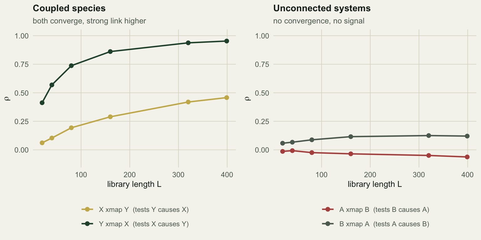
“Y xmap X” climbs from 0.413 at L = 20 to 0.953 at the full library: strong, converging evidence that X drives Y. “X xmap Y” climbs from 0.061 to 0.458: weaker, but also converging, and Y does affect X, at one fifth the strength. The ranking of the two curves matches the ranking of the two coefficients, from series that correlate at 0.11.

The right panel is two chaotic populations from completely separate systems. Their cross maps sit at zero and stay there at every library length. Nothing to find, nothing found.

Convergence is the test

The single most common misuse of CCM is to run it once, at the full library, get a decent correlation, and call it causation. The next demonstration is why that fails.

Two species that never interact, both responding to the same environmental driver:

set.seed(6266)
z_drv <- gen_ricker(n)                                # shared driver
r1 <- as.numeric(2.0 * scale(z_drv)) + rnorm(n, 0, 0.3)
r2 <- as.numeric(1.5 * scale(z_drv)) + rnorm(n, 0, 0.3)

r_shared <- cor(r1, r2)
ccm_12 <- ccm_curve(r1, r2, E = 2, lib_sizes = Ls)
ccm_21 <- ccm_curve(r2, r1, E = 2, lib_sizes = Ls)
delta_12 <- ccm_12[length(Ls)] - ccm_12[1]
delta_YX <- ccm_YX[length(Ls)] - ccm_YX[1]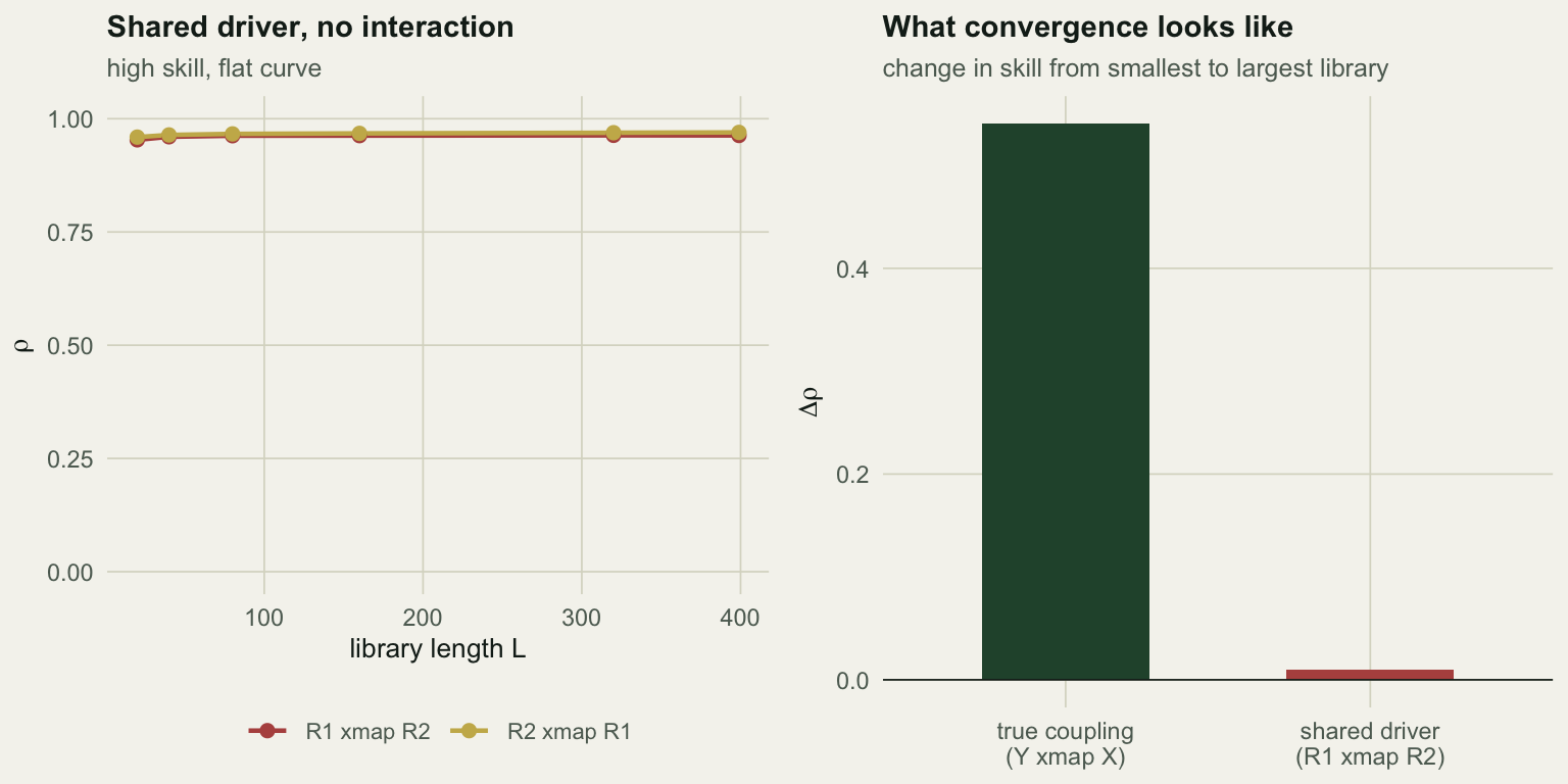

Figure 2: Two species responding to a shared driver but not to each other. Cross-map skill is high at every library length and does not rise, which is the signature of common forcing rather than causation.

R1 and R2 correlate at 0.97 and cross-map each other at 0.963. Reported at the full library alone, that is an overwhelming result for a link that does not exist.

The curve is what saves you. Skill rises by +0.010 from the smallest to the largest library: it is already saturated at L = 20 because R1 and R2 are just smooth functions of the same thing, and twenty points are enough to learn a smooth function. Genuine dynamical coupling behaves differently, because the estimate depends on finding nearby states on an attractor, and that only gets easier as the library fills. The true coupling gained +0.540 over the same range.

So the quantity to report is not rho. It is rho as a function of L, and the increase across it.

Putting a number on it

A rising curve still needs a null, because autocorrelated series can drift upward for uninteresting reasons. The right null keeps the linear structure of the series and destroys everything else: the phase-randomised surrogate, which preserves the power spectrum exactly and randomises the Fourier phases.

surrogate_ebi <- function(x) {
  n <- length(x); xm <- mean(x); z <- x - xm
  f <- fft(z); amp <- Mod(f)
  nyq <- floor(n / 2)
  newf <- complex(modulus = amp, argument = 0)
  ph <- runif(nyq - 1, 0, 2 * pi)
  newf[2:nyq] <- complex(modulus = amp[2:nyq], argument = ph)
  newf[n:(n - nyq + 2)] <- Conj(newf[2:nyq])          # keep the series real
  newf[1] <- f[1]
  if (n %% 2 == 0)
    newf[nyq + 1] <- complex(modulus = amp[nyq + 1],
                             argument = ifelse(runif(1) < 0.5, 0, pi))
  Re(fft(newf, inverse = TRUE)) / n + xm
}

set.seed(8266)
obs_delta <- delta_YX
null_delta <- replicate(100, {
  xs <- surrogate_ebi(d$x)
  lo <- mean(replicate(6, ccm_once(d$y, xs, E = 2, lib_size = Ls[1])), na.rm = TRUE)
  hi <- mean(replicate(6, ccm_once(d$y, xs, E = 2, lib_size = Ls[length(Ls)])), na.rm = TRUE)
  hi - lo
})
p_conv <- mean(null_delta >= obs_delta)
null_q95 <- quantile(null_delta, 0.95)

The observed increase for “Y xmap X” is +0.540. Against 100 surrogates of X with an identical power spectrum, the 95th percentile of the null increase is +0.129, and the observed value is exceeded by 0% of them. The convergence is not something autocorrelation alone produces.

Note what the surrogate is doing. It leaves X’s autocorrelation, spectrum and marginal spread alone, and scrambles only the deterministic trajectory. If the cross map were picking up “X is a smooth wiggly thing and so is Y”, the surrogates would reproduce it. They do not.

What this does not give you

CCM answers a narrow question well: does the reconstruction of Y contain the signature of X, more and more clearly as the library grows? Several things follow, and several do not.

• Both directions can converge, and here both should, because the true system is bidirectionally coupled. The asymmetry is the useful output: 0.953 against 0.458, matching a fivefold difference in coupling. Do not read a converging weak direction as “no effect”.
• The skill ceiling is not an effect size. How high a converging curve reaches depends on process noise, observation error, series length and how much of the driven species’ variance the driver explains. Two systems with identical coupling strengths can plateau at different heights.
• A shared driver lifts the cross map between two species that never touch. Above, the driver was copied straight into both series. When it enters their dynamics instead, the cross map runs at a moderate skill in both directions and does not converge, so the test still gives the right answer: convergence is what protects you, and reporting rho alone is what throws that protection away. The checking post works through that case, and a harder one: when the forcing is strong enough to synchronise the two species, the true direction stops converging as well.
• Nothing here needs the coupling to be linear, and nothing here tests a mechanism. X drives Y is a statement about dynamics, not about how. Competition, predation, and a shared pathogen all leave the same trace.
• It needs a long, well-sampled series. Four hundred points from a noiseless map is a friendly case. Real ecological series are shorter and dirtier, and the convergence test is the first thing to go.

Where to go next

The method is not exotic. It is simplex projection pointed at a neighbouring variable, plus one deliberately chosen sweep over library length, plus a surrogate null. Everything in this post is base R and about sixty lines.

The seduction is in how good the output looks. A converging curve with a surrogate p-value is a persuasive figure, and it can be produced by systems with no link between the two species at all. Before running this on your own data, work through what breaks it.

References

Sugihara, May, Ye, Hsieh, Deyle, Fogarty & Munch 2012 Science 338(6106):496-500 (10.1126/science.1227079)

Takens 1981 Lecture Notes in Mathematics 898:366-381 (10.1007/BFb0091924)

Ye, Deyle, Gilarranz & Sugihara 2015 Scientific Reports 5:14750 (10.1038/srep14750)

Granger 1969 Econometrica 37(3):424-438 (10.2307/1912791)

Deyle, Fogarty, Hsieh, Kaufman, MacCall, Munch, Perretti, Ye & Sugihara 2013 Proceedings of the National Academy of Sciences 110(16):6430-6435 (10.1073/pnas.1215506110)

Clark, Ye, Isbell, Deyle, Cowles, Tilman & Sugihara 2015 Ecology 96(5):1174-1181 (10.1890/14-1479.1)

Ebisuzaki 1997 Journal of Climate 10(9):2147-2153

Related tutorials

• Simplex projection and delay embedding
• The S-map and state-dependent dynamics
• Checking an empirical dynamic model
• Confounding and backdoor adjustment