---
title: "Confounding and backdoor adjustment"
description: "Why a naive regression gives a biased causal effect in ecology, and how the backdoor criterion says which covariates to adjust for and which to leave out."
date: "2026-05-25 11:00"
categories: [causal inference, R, ecology tutorial, regression, DAGs]
image: thumbnail.png
image-alt: "Two overlaid sampling distributions, the naive estimator shifted away from the dashed true-effect line and the adjusted estimator centred on it."
date-modified: "2026-09-27"
---
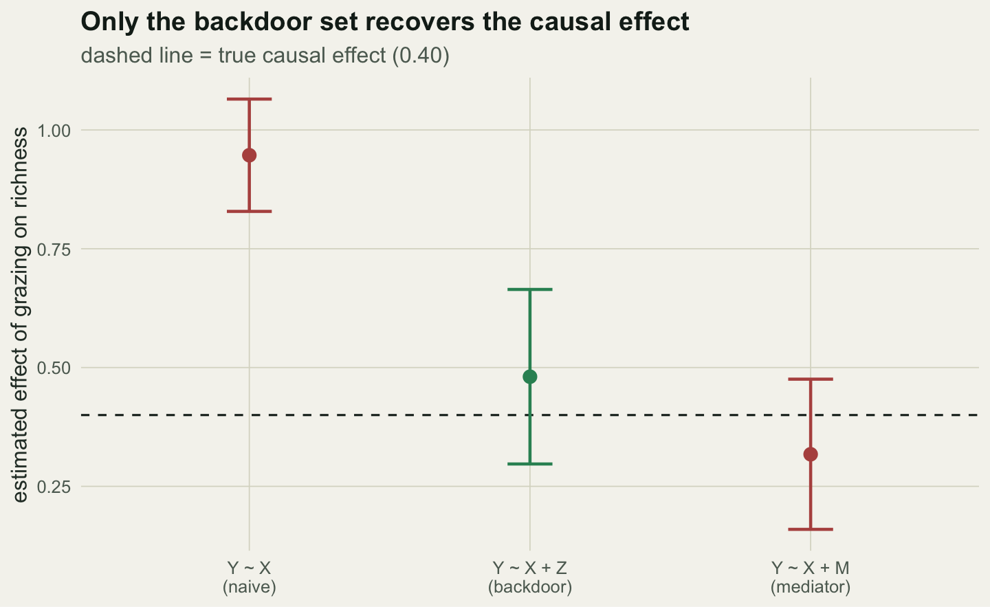
*Corrected 27 September 2026: the estimates figure judged the mediator model against the grazing effect of 0.40, which is not a true value in its separate simulation; it now shows that model against its own total effect of 0.72, which its interval misses.*
Fit `richness ~ grazing` and you get a slope. Call it the effect of grazing on richness and you have quietly assumed something the regression never checked: that nothing else drives both. In observational ecology something usually does. A productive soil can raise grazing pressure and, separately, support more species; the raw slope then mixes the grazing effect with the soil gradient that produced it. The estimate is precise and wrong.
This is confounding, and it has a graphical solution. A directed acyclic graph (DAG) writes down which variable causes which, and the backdoor criterion reads off the graph the exact set of covariates you must adjust for to isolate one causal effect. Adjust for that set and the bias closes. Adjust for the wrong things and, as the next post shows, you can open bias that was not there. This post stays with the first case: a genuine confounder, the backdoor adjustment that removes it, and the honest limit that no adjustment can pass.
## A confounded slope
Let `X` be grazing intensity, `Y` plant species richness, and `Z` soil productivity. Productivity drives both: it pushes grazing up (`Z -> X`) and richness up (`Z -> Y`). Grazing also has its own, smaller effect on richness (`X -> Y`), which is what we actually want. The path `X <- Z -> Y` is a backdoor: a non-causal route connecting `X` and `Y` through their common cause. A regression of `Y` on `X` alone travels that route and adds it to the answer.
```{r}
#| label: setup
#| code-fold: true
#| code-summary: "Setup: packages, colours and plot theme"
#| results: hide
#| message: false
#| warning: false
library(ggplot2)
paper <- "#f5f4ee"; ink <- "#16241d"; body <- "#2c3a31"
forest <- "#275139"; faint <- "#5d6b61"; line_col <- "#dad9ca"
red <- "#b5534e"; green <- "#2f8f63"
theme_te <- function(base_size = 12){
  theme_minimal(base_size = base_size) +
    theme(plot.background = element_rect(fill = paper, colour = NA),
          panel.background = element_rect(fill = paper, colour = NA),
          panel.grid.minor = element_blank(),
          panel.grid.major = element_line(colour = line_col, linewidth = 0.3),
          text = element_text(colour = body),
          plot.title = element_text(colour = ink, face = "bold"),
          plot.subtitle = element_text(colour = faint),
          axis.text = element_text(colour = faint),
          legend.position = "top")
}
```
```{r}
#| label: confounded-fit
set.seed(159)
n   <- 300
bX  <- 0.40                 # true causal effect of grazing on richness
bZ  <- 0.60                 # soil productivity -> richness
aZX <- 0.80                 # soil productivity -> grazing
Z <- rnorm(n)
X <- aZX * Z + rnorm(n, 0, 0.6)
Y <- bX * X + bZ * Z + rnorm(n, 0, 1)

m_naive <- lm(Y ~ X)        # travels the backdoor X <- Z -> Y
m_adj   <- lm(Y ~ X + Z)    # blocks it by conditioning on Z

est_naive <- coef(m_naive)["X"]; ci_naive <- confint(m_naive)["X", ]
est_adj   <- coef(m_adj)["X"];   ci_adj   <- confint(m_adj)["X", ]
```
The true grazing effect is `r bX`. The naive slope comes out at `r round(est_naive, 3)`, with a 95% interval of [`r round(ci_naive[1], 2)`, `r round(ci_naive[2], 2)`] that does not come close to the truth. Conditioning on productivity gives `r round(est_adj, 3)`, interval [`r round(ci_adj[1], 2)`, `r round(ci_adj[2], 2)`], which covers it. The bias is not a small-sample accident; it is structural. The population slope of the naive fit is `r bX` plus the backdoor contribution `bZ * cov(X, Z) / var(X)`:
```{r}
#| label: analytic
naive_pop <- bX + bZ * (cov(X, Z) / var(X))
```
which evaluates to `r round(naive_pop, 3)`. More data buys you a tighter interval around the wrong number.
```{r}
#| label: fig-estimates
#| fig-cap: "Estimated grazing effect from three models, with 95% intervals. Only the backdoor-adjusted model is unbiased for the true effect (dashed line). The mediator model comes from a separate simulation whose total effect is the dotted line; conditioning on the mediator removes part of that effect on purpose."
#| fig-alt: "A dot-and-interval plot of three estimates. The naive model sits far above a dashed line at 0.40 and the backdoor model sits on it; the mediator model, from a separate simulation, sits far below its own dotted total-effect line at 0.72."
#| fig-width: 7.5
#| fig-height: 4.6
set.seed(1590)
n2 <- 300
Xm <- rnorm(n2)
M  <- 0.7 * Xm + rnorm(n2, 0, 0.7)          # X -> M
Ym <- 0.3 * Xm + 0.6 * M + rnorm(n2, 0, 1)  # X -> Y (direct) and M -> Y
total_true <- 0.3 + 0.7 * 0.6
m_med <- lm(Ym ~ Xm + M)                     # conditions on a mediator
est_med <- coef(m_med)["Xm"]; ci_med <- confint(m_med)["Xm", ]

fig1 <- data.frame(
  model = factor(c("Y ~ X\n(naive)", "Y ~ X + Z\n(backdoor)", "Y ~ X + M\n(mediator)"),
                 levels = c("Y ~ X\n(naive)", "Y ~ X + Z\n(backdoor)", "Y ~ X + M\n(mediator)")),
  est = c(est_naive, est_adj, est_med),
  lo  = c(ci_naive[1], ci_adj[1], ci_med[1]),
  hi  = c(ci_naive[2], ci_adj[2], ci_med[2]),
  kind = c("wrong", "right", "wrong"))
ggplot(fig1, aes(model, est, colour = kind)) +
  scale_x_discrete() +
  annotate("segment", x = 0.6, xend = 2.4, y = bX, yend = bX, linetype = "dashed", colour = ink) +
  annotate("segment", x = 2.6, xend = 3.4, y = total_true, yend = total_true,
           linetype = "dotted", colour = ink, linewidth = 0.8) +
  geom_errorbar(aes(ymin = lo, ymax = hi), width = 0.16, linewidth = 0.8) +
  geom_point(size = 3) +
  scale_colour_manual(values = c(right = green, wrong = red), guide = "none") +
  labs(x = NULL, y = "estimated effect of grazing on richness",
       title = "Only the backdoor set recovers the causal effect",
       subtitle = "dashed = true grazing effect (0.40)\ndotted = total effect in the mediator simulation (0.72)") +
  theme_te()
```
## Adjust for confounders, not for everything
A tempting shortcut is to throw every available covariate into the model. That is not what the backdoor criterion says, and the third bar above shows why. Suppose grazing affects richness partly through a mediator `M`, some intermediate on the path `X -> M -> Y` (say sward height). The total causal effect of grazing is the sum of its direct effect and everything routed through `M`, here `r round(total_true, 2)`. Conditioning on `M` holds the mediator fixed and reports only the leftover direct piece, `r round(est_med, 3)`: a real quantity, but not the total effect, and badly wrong if the total is what the question asked for. Mediators, colliders, and instruments each demand different handling; a covariate is not a free win just because it is available and correlated. The graph is what tells them apart, and drawing the direct-versus-indirect split explicitly is the job of a [path model](../path-analysis-direct-indirect-effects/).
## The bias is systematic, not noise
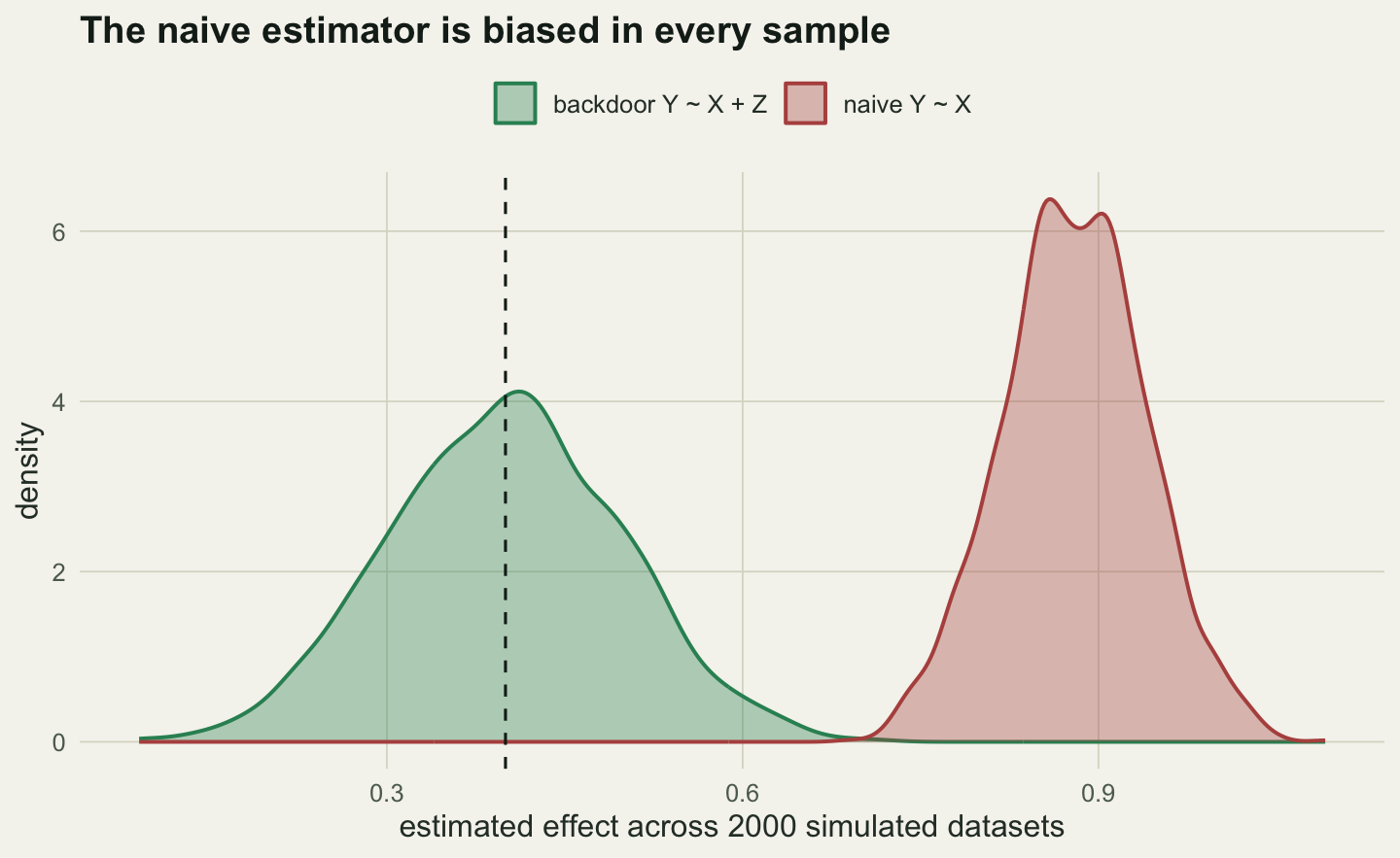
To see that the naive estimator is biased rather than merely variable, refit both models on many fresh datasets and record how often each 95% interval traps the truth.
```{r}
#| label: coverage
set.seed(20159)
nsim <- 2000
est_n <- est_a <- numeric(nsim)
cov_n <- cov_a <- logical(nsim)
for (i in seq_len(nsim)) {
  Zi <- rnorm(n); Xi <- aZX * Zi + rnorm(n, 0, 0.6)
  Yi <- bX * Xi + bZ * Zi + rnorm(n)
  mn <- lm(Yi ~ Xi); ma <- lm(Yi ~ Xi + Zi)
  est_n[i] <- coef(mn)["Xi"]; est_a[i] <- coef(ma)["Xi"]
  cn <- confint(mn)["Xi", ]; ca <- confint(ma)["Xi", ]
  cov_n[i] <- bX >= cn[1] && bX <= cn[2]
  cov_a[i] <- bX >= ca[1] && bX <= ca[2]
}
```
The naive estimator averages `r round(mean(est_n), 3)` (a bias of `r sprintf("%+.3f", mean(est_n) - bX)`) and its interval covers the truth in `r round(100 * mean(cov_n), 1)`% of samples: never. The adjusted estimator averages `r round(mean(est_a), 3)`, essentially unbiased, and covers at `r round(100 * mean(cov_a), 1)`%, near the nominal rate. Confounding does not average out.
```{r}
#| label: fig-coverage
#| fig-cap: "Sampling distributions of the two estimators over 2000 simulated datasets. The naive estimator is displaced from the truth in essentially every sample; the backdoor-adjusted estimator is centred on it."
#| fig-alt: "Two density curves over the estimate axis. The naive curve is centred near 0.88, the backdoor curve near 0.40 at the dashed true-effect line, with little overlap."
#| fig-width: 7.5
#| fig-height: 4.6
dd <- rbind(data.frame(est = est_n, estimator = "naive Y ~ X"),
            data.frame(est = est_a, estimator = "backdoor Y ~ X + Z"))
ggplot(dd, aes(est, fill = estimator, colour = estimator)) +
  geom_density(alpha = 0.35, linewidth = 0.7) +
  geom_vline(xintercept = bX, linetype = "dashed", colour = ink) +
  scale_fill_manual(values = c("naive Y ~ X" = red, "backdoor Y ~ X + Z" = green)) +
  scale_colour_manual(values = c("naive Y ~ X" = red, "backdoor Y ~ X + Z" = green)) +
  labs(x = "estimated effect across 2000 simulated datasets", y = "density",
       title = "The naive estimator is biased in every sample",
       fill = NULL, colour = NULL) +
  theme_te()
```
## The honest limit
The adjusted model is only as good as the graph behind it. The backdoor criterion guarantees an unbiased effect when the adjustment set blocks every backdoor path, which presumes you have named and measured every common cause. Miss one, and an unmeasured confounder reopens a backdoor that conditioning on `Z` cannot touch. No amount of data reveals the omission: the fit looks clean, the interval looks tight, and the number is still biased by however much the missing cause contributed. This is the standing caveat of all observational causal work, and it cannot be tested from the data alone; it can only be probed, which is the subject of [checking causal assumptions](../checking-causal-assumptions/). Adjustment turns a stated set of assumptions into an estimate. It does not verify the assumptions, and it is worth being explicit about which ones you are asking the reader to grant.
## References
Arif S, MacNeil MA 2022. Ecology Letters 25(8):1741-1745 (10.1111/ele.14033).
Arif S, MacNeil MA 2023. Ecological Monographs 93(1):e1554 (10.1002/ecm.1554).
Greenland S, Pearl J, Robins JM 1999. Epidemiology 10(1):37-48 (10.1097/00001648-199901000-00008).
Pearl J 2009. Causality: Models, Reasoning and Inference, 2nd ed. Cambridge University Press (ISBN 978-0-521-89560-6).
Pearl J, Glymour M, Jewell NP 2016. Causal Inference in Statistics: A Primer. Wiley (ISBN 978-1-119-18684-7).
Textor J, van der Zander B, Gilthorpe MS, Liskiewicz M, Ellison GTH 2016. International Journal of Epidemiology 45(6):1887-1894 (10.1093/ije/dyw341).
## Related tutorials
- [Collider bias and selection](../collider-bias-and-selection/)
- [Checking causal assumptions](../checking-causal-assumptions/)
- [Front-door adjustment when no instrument exists](../front-door-adjustment/)
- [Lasso, stepwise and the dropped confounder](../lasso-drops-the-confounder/)