---
title: "Collider bias and selection"
description: "Conditioning on a common effect, or sampling on it, manufactures an ecological correlation that is not there. Why adjusting for everything is a bad instinct."
date: "2026-05-25 12:00"
categories: [causal inference, R, ecology tutorial, regression, DAGs]
image: thumbnail.png
image-alt: "Two scatter panels of the same two traits: flat and uncorrelated in the whole population, sloping downward in the detected sample only."
---
The previous post made adjustment look like a cure: name the confounder, put it in the model, close the backdoor. That invites a dangerous generalisation, that more covariates are always safer. They are not. There is a second kind of variable that does the opposite of a confounder, and conditioning on it opens a path that was closed. A regression that adjusts for it does not remove bias; it invents an association from nothing.
That variable is a collider: a common effect of two others. If body size and boldness both raise an animal's chance of being trapped, then size and boldness are the collider's parents and capture is the collider. In the population the two traits may be unrelated. Restrict attention to the trapped sample, or put capture in a regression, and a spurious trade-off appears. This is not a small correction. It fabricates effects that are large, highly significant, and entirely artefactual.
## An association from nothing
Let `X` and `Y` be two traits with no causal link between them, and let a collider `C` be a common effect of both. Regressing `Y` on `X` alone correctly finds nothing. Add `C` to the model and the picture changes.
```{r}
#| label: setup
#| code-fold: true
#| code-summary: "Setup: packages, colours and plot theme"
#| results: hide
#| message: false
#| warning: false
library(ggplot2)
paper <- "#f5f4ee"; ink <- "#16241d"; body <- "#2c3a31"
forest <- "#275139"; faint <- "#5d6b61"; line_col <- "#dad9ca"
red <- "#b5534e"; green <- "#2f8f63"
theme_te <- function(base_size = 12){
  theme_minimal(base_size = base_size) +
    theme(plot.background = element_rect(fill = paper, colour = NA),
          panel.background = element_rect(fill = paper, colour = NA),
          panel.grid.minor = element_blank(),
          panel.grid.major = element_line(colour = line_col, linewidth = 0.3),
          text = element_text(colour = body),
          plot.title = element_text(colour = ink, face = "bold"),
          plot.subtitle = element_text(colour = faint),
          axis.text = element_text(colour = faint),
          strip.text = element_text(colour = ink, face = "bold"),
          legend.position = "top")
}
```
```{r}
#| label: collider-continuous
set.seed(160)
n <- 2000
X <- rnorm(n)                       # trait 1, no link to Y
Y <- rnorm(n)                       # trait 2
C <- X + Y + rnorm(n, 0, 0.5)       # a common effect of both

m_correct  <- lm(Y ~ X)             # correct: leaves the collider alone
m_collider <- lm(Y ~ X + C)         # wrong: conditions on the collider
b_corr <- coef(m_correct)["X"];  ci_corr <- confint(m_correct)["X", ]
b_coll <- coef(m_collider)["X"]; ci_coll <- confint(m_collider)["X", ]
```
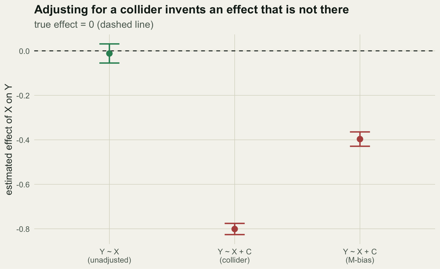
The two traits are genuinely unrelated: their sample correlation is `r round(cor(X, Y), 3)` and the plain regression slope is `r round(b_corr, 3)`, interval [`r round(ci_corr[1], 2)`, `r round(ci_corr[2], 2)`]. Condition on the collider and the estimated effect of `X` on `Y` swings to `r round(b_coll, 3)`, interval [`r round(ci_coll[1], 2)`, `r round(ci_coll[2], 2)`]: a strong, tightly estimated relationship between two variables that have nothing to do with each other. Holding `C` fixed forces a trade-off, because a high `C` reached with a low `X` implies a high `Y`.
## Selection is conditioning in disguise
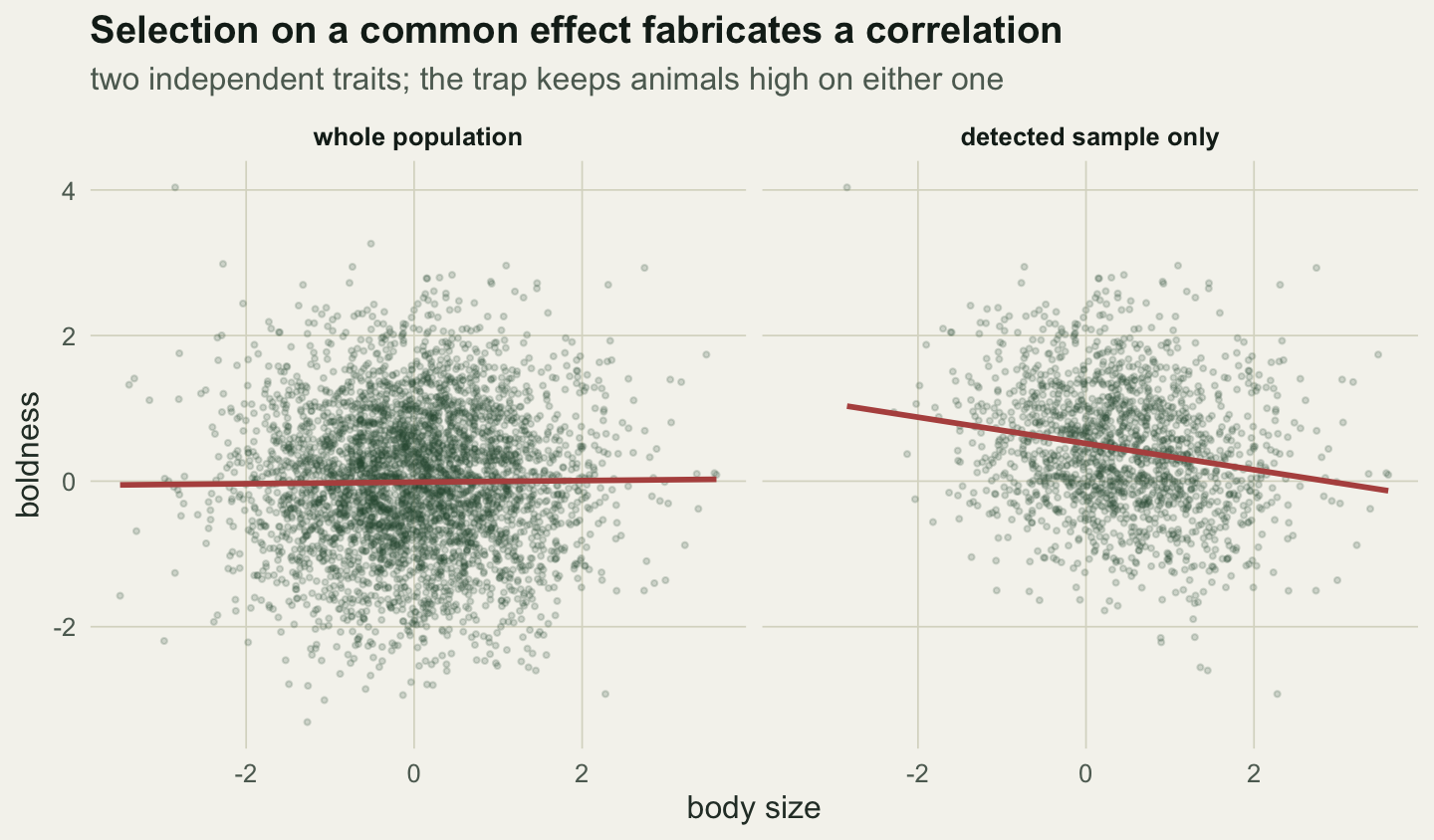
You do not need to put the collider in a model to suffer for it. Sampling on a common effect does the same thing, quietly, before any regression is fitted. Suppose body size and boldness independently raise capture probability, and you only ever measure trapped animals.
```{r}
#| label: fig-collider-scatter
#| fig-cap: "Two independent traits, in the whole population and in the trapped sample. Both traits raise capture probability, so the trap retains animals high on one or the other; the survivors show a trade-off that does not exist in the population."
#| fig-alt: "Left panel: a round cloud of points with a flat red fit line. Right panel: the retained subset, thinned at the bottom-left, with a downward-sloping red fit line."
#| fig-width: 7.5
#| fig-height: 4.4
set.seed(1600)
npop <- 4000
Xs <- rnorm(npop)                    # body size
Ys <- rnorm(npop)                    # boldness (independent of size)
det <- rbinom(npop, 1, plogis(-0.4 + 1.2 * Xs + 1.2 * Ys)) == 1
cor_full <- cor(Xs, Ys); cor_det <- cor(Xs[det], Ys[det])

d1 <- rbind(data.frame(x = Xs, y = Ys, set = "whole population"),
            data.frame(x = Xs[det], y = Ys[det], set = "detected sample only"))
d1$set <- factor(d1$set, levels = c("whole population", "detected sample only"))
ggplot(d1, aes(x, y)) +
  geom_point(alpha = 0.18, colour = forest, size = 0.7) +
  geom_smooth(method = "lm", formula = y ~ x, se = FALSE, colour = red, linewidth = 1) +
  facet_wrap(~set) +
  labs(x = "body size", y = "boldness",
       title = "Selection on a common effect fabricates a correlation",
       subtitle = "two independent traits; the trap keeps animals high on either one") +
  theme_te()
```
In the whole population the traits correlate at `r round(cor_full, 3)`, essentially zero. Among the `r sum(det)` trapped animals, out of `r npop`, the correlation is `r round(cor_det, 3)`: a clear apparent trade-off, produced entirely by who ended up in the sample. Survivorship, detection filters, and museum collections all select on traits that also affect the response, and each one is a collider waiting to bias the analysis. The problem is baked into the data before you open R.
## The pre-treatment trap
The habit worth unlearning is adjusting for a covariate just because it was measured before the treatment and looks harmless. Pre-treatment covariates can be colliders too. Consider two hidden causes `U1` and `U2`, a covariate `C` that both influence, a treatment `X` driven by `U1`, and an outcome `Y` driven by `U2`. There is no causal path from `X` to `Y`, and no ordinary confounding of the two. Adjust for `C` anyway and you open the route `X` from `U1` into `C` and out through `U2` to `Y`.
```{r}
#| label: m-bias
set.seed(16000)
nm <- 3000
U1 <- rnorm(nm); U2 <- rnorm(nm)
Xm <- 0.9 * U1 + rnorm(nm, 0, 0.6)                 # X <- U1
Cm <- 0.9 * U1 + 0.9 * U2 + rnorm(nm, 0, 0.6)      # C <- U1, C <- U2 (pre-treatment)
Ym <- 0.9 * U2 + rnorm(nm, 0, 0.6)                 # Y <- U2
m_corr2 <- lm(Ym ~ Xm);      b_m_corr <- coef(m_corr2)["Xm"]
m_mbias <- lm(Ym ~ Xm + Cm); b_m_coll <- coef(m_mbias)["Xm"]; ci_m_coll <- confint(m_mbias)["Xm", ]
```
Left alone, `X` and `Y` are unrelated: the slope is `r round(b_m_corr, 3)`. Adjust for the pre-treatment covariate `C` and it becomes `r round(b_m_coll, 3)`, interval [`r round(ci_m_coll[1], 2)`, `r round(ci_m_coll[2], 2)`]. This is M-bias, and it is the sharpest warning against reflexive adjustment: the covariate is measured first, is correlated with both treatment and outcome, and putting it in the model is exactly what creates the bias. Only the graph distinguishes a confounder to include from a collider to leave out; correlation with the variables of interest does not.
```{r}
#| label: fig-collider-estimates
#| fig-cap: "Estimated effect of X on Y under three models. The true effect is zero (dashed line). Leaving the collider alone recovers it; conditioning on the collider, or on the pre-treatment collider that drives M-bias, fabricates a strong negative effect."
#| fig-alt: "A dot-and-interval plot against a dashed line at zero. The unadjusted estimate sits on the line; the collider and M-bias estimates sit well below it with tight intervals."
#| fig-width: 7.5
#| fig-height: 4.6
fig2 <- data.frame(
  model = factor(c("Y ~ X\n(unadjusted)", "Y ~ X + C\n(collider)", "Y ~ X + C\n(M-bias)"),
                 levels = c("Y ~ X\n(unadjusted)", "Y ~ X + C\n(collider)", "Y ~ X + C\n(M-bias)")),
  est = c(b_corr, b_coll, b_m_coll),
  lo  = c(ci_corr[1], ci_coll[1], ci_m_coll[1]),
  hi  = c(ci_corr[2], ci_coll[2], ci_m_coll[2]),
  kind = c("right", "wrong", "wrong"))
ggplot(fig2, aes(model, est, colour = kind)) +
  geom_hline(yintercept = 0, linetype = "dashed", colour = ink) +
  geom_errorbar(aes(ymin = lo, ymax = hi), width = 0.16, linewidth = 0.8) +
  geom_point(size = 3) +
  scale_colour_manual(values = c(right = green, wrong = red), guide = "none") +
  labs(x = NULL, y = "estimated effect of X on Y",
       title = "Adjusting for a collider invents an effect that is not there",
       subtitle = "true effect = 0 (dashed line)") +
  theme_te()
```
## Fabrication, not noise
Colliders do not merely add variance; they produce a consistent false signal that a significance test then rubber-stamps. Refit the true null many times and count how often each model rejects it.
```{r}
#| label: type-one
set.seed(21600)
nsim <- 2000; nn <- 300
sig_un <- sig_co <- sig_mb <- logical(nsim)
for (i in seq_len(nsim)) {
  x <- rnorm(nn); y <- rnorm(nn); cc <- x + y + rnorm(nn, 0, 0.5)
  sig_un[i] <- summary(lm(y ~ x))$coefficients["x", "Pr(>|t|)"] < 0.05
  sig_co[i] <- summary(lm(y ~ x + cc))$coefficients["x", "Pr(>|t|)"] < 0.05
  u1 <- rnorm(nn); u2 <- rnorm(nn)
  xm <- 0.9 * u1 + rnorm(nn, 0, 0.6)
  cm <- 0.9 * u1 + 0.9 * u2 + rnorm(nn, 0, 0.6)
  ym <- 0.9 * u2 + rnorm(nn, 0, 0.6)
  sig_mb[i] <- summary(lm(ym ~ xm + cm))$coefficients["xm", "Pr(>|t|)"] < 0.05
}
```
The unadjusted model rejects the true null in `r round(100 * mean(sig_un), 1)`% of samples, the nominal 5%. The collider model rejects in `r round(100 * mean(sig_co), 1)`% and the M-bias model in `r round(100 * mean(sig_mb), 1)`%: a fabricated effect is found in essentially every sample. A tight confidence interval and a small p-value describe how reliably the artefact reproduces, not whether it is real.
## The honest limit
There is no data-only test that separates a confounder from a collider. Both are correlated with the treatment and the outcome; the difference lies entirely in the direction of the arrows, which the data do not carry. This is the same wall met by [d-separation](../piecewise-sem-d-separation/) and [Markov equivalence](../checking-a-structural-equation-model/): the numbers fix the associations, not the causal roles behind them. Deciding what to adjust for is therefore a modelling decision made before the regression, from a stated causal graph, not a search over which covariates tighten the fit. Adjust for the backdoor set, and nothing else.
## References
Berkson J 1946. Biometrics Bulletin 2(3):47-53 (10.2307/3002000).
Cole SR, Platt RW, Schisterman EF, Chu H, Westreich D, Richardson D, Poole C 2010. International Journal of Epidemiology 39(2):417-420 (10.1093/ije/dyp334).
Elwert F, Winship C 2014. Annual Review of Sociology 40:31-53 (10.1146/annurev-soc-071913-043455).
Greenland S, Pearl J, Robins JM 1999. Epidemiology 10(1):37-48 (10.1097/00001648-199901000-00008).
Munafo MR, Tilling K, Taylor AE, Evans DM, Davey Smith G 2018. International Journal of Epidemiology 47(1):226-235 (10.1093/ije/dyx206).
Pearl J 2009. Causality: Models, Reasoning and Inference, 2nd ed. Cambridge University Press (ISBN 978-0-521-89560-6).
## Related tutorials
- [Confounding and backdoor adjustment](../confounding-and-backdoor-adjustment/)
- [Parasite burdens truncated by host death](../truncated-parasite-burden/)
- [Attrition in a field experiment: when pots die first](../attrition-in-a-field-experiment/)
- [Non-compliance in field experiments](../non-compliance-in-field-experiments/)