library(ggplot2)

te <- list(paper="#f5f4ee", card="#ffffff", ink="#16241d", body="#2c3a31",
           forest="#275139", label="#46604a", sage="#93a87f", line="#dad9ca",
           muted="#5d6b61", warm="#b5534e", gold="#cda23f")

theme_te <- function(base_size = 12) {
  theme_minimal(base_size = base_size) +
    theme(plot.background  = element_rect(fill = te$paper, colour = NA),
          panel.background = element_rect(fill = te$paper, colour = NA),
          panel.grid.major = element_line(colour = te$line, linewidth = 0.3),
          panel.grid.minor = element_blank(),
          axis.text  = element_text(colour = te$muted, size = base_size * 0.85),
          axis.title = element_text(colour = te$body),
          plot.title = element_text(colour = te$ink, face = "bold", size = base_size * 1.1),
          plot.subtitle = element_text(colour = te$muted, size = base_size * 0.9),
          strip.text = element_text(colour = te$ink, face = "bold"),
          legend.text = element_text(colour = te$body))
}

knitr::opts_chunk$set(fig.align = "center", dev = "png", dpi = 150)Piecewise SEM and the test of d-separation
R
structural equation models
model diagnostics
GLM
ecology tutorial
Fit a structural equation model equation by equation with lm and glm, then test its causal structure with Shipley’s d-separation test and Fisher’s C in base R.
The classical way to fit a structural equation model compares an observed covariance matrix with the one a model implies, and estimates every path at once by maximum likelihood. It is elegant, but it assumes multivariate normality and struggles the moment a response is a count, a proportion, or comes from nested sampling. Piecewise SEM takes a different route (Shipley 2009, Lefcheck 2016): estimate each equation locally with whatever model suits that response, a glm for counts, an lm for a Gaussian variable, a mixed model for nested data. That flexibility raises an awkward question. If the model is a collection of separate regressions, how do you test the model as a whole?
The answer is the test of directed separation (Shipley 2000). A directed acyclic graph implies a specific list of conditional independences: any two variables with no arrow between them must be independent once you condition on the right set. Test each of those claims, combine the p-values, and you have a single goodness-of-fit test for the entire causal structure, one that works no matter what distributions the equations use.
The idea in one paragraph
Two variables that are not directly connected in the graph should carry no residual association after conditioning on the parents of either. That is a testable claim: regress the later variable on the earlier one plus the conditioning set, and look at the p-value of the earlier variable. The full set of such claims for all non-adjacent pairs is the basis set. Shipley combines their p-values with Fisher’s statistic, C = -2 times the sum of the log p-values, which follows a chi-squared distribution with 2k degrees of freedom for k claims. A large C (small upper-tail probability) means at least one implied independence is violated, so the structure is wrong.
An ecological graph with a count response
The data are synthetic and illustrative. Elevation lowers temperature; temperature raises vegetation cover; and insect abundance, a count, depends on both vegetation and temperature directly. That last detail matters: it is a direct arrow that a careless diagram might drop.
set.seed(156)
n <- 200
elevation <- rnorm(n)
temp <- -0.70 * elevation + sqrt(1 - 0.7^2) * rnorm(n)   # colder at height
veg  <-  0.60 * temp      + sqrt(1 - 0.6^2) * rnorm(n)   # warmer, more cover
eta  <- 0.30 + 0.55 * veg + 0.45 * temp                 # insects depend on both
insects <- rpois(n, exp(eta))
dat <- data.frame(elevation, temp, veg, insects)
Each equation is fitted with the model its response deserves: two Gaussian lm fits, and a Poisson glm for the count.
m_temp <- lm(temp ~ elevation)
m_veg  <- lm(veg ~ temp)
m_ins  <- glm(insects ~ veg + temp, family = poisson)

b_et <- unname(coef(m_temp)["elevation"])
b_tv <- unname(coef(m_veg)["temp"])
b_vi <- unname(coef(m_ins)["veg"])
b_ti <- unname(coef(m_ins)["temp"])
disp <- sum(residuals(m_ins, "pearson")^2) / m_ins$df.residual
The fitted paths are elevation to temperature -0.65, temperature to vegetation 0.58, and on the log scale of the count, vegetation to insects 0.6 and temperature to insects 0.4. The Poisson fit is well behaved (Pearson dispersion 0.77). Every path is clearly supported, and someone checking each equation on its own would see nothing wrong. The test below asks a question the individual equations cannot: is anything missing?
Testing the basis set
Two small helpers do the work. The first tests one independence claim by regressing the response on the conditioning set plus the predictor of interest and returning that predictor’s p-value; it takes a family argument so a count claim uses a Poisson glm. The second combines a vector of claim p-values into Fisher’s C.
claim_p <- function(resp, pred, cond, family = c("gaussian","poisson")) {
  family <- match.arg(family)
  f <- as.formula(paste(resp, "~", paste(c(pred, cond), collapse = " + ")))
  m <- if (family == "gaussian") lm(f, data = dat) else glm(f, family = poisson, data = dat)
  co <- summary(m)$coefficients
  co[pred, ncol(co)]           # last column: Pr(>|t|) or Pr(>|z|)
}
fishersC <- function(ps) {
  C <- -2 * sum(log(ps)); df <- 2 * length(ps)
  c(C = C, df = df, p = pchisq(C, df, lower.tail = FALSE))
}
The true graph has arrows elevation to temp, temp to veg, temp to insects, veg to insects. The non-adjacent pairs are (elevation, vegetation) and (elevation, insects), so the basis set has two claims.
pA1 <- claim_p("veg", "elevation", "temp", "gaussian")               # elev _||_ veg | temp
pA2 <- claim_p("insects", "elevation", c("veg","temp"), "poisson")   # elev _||_ ins | veg, temp
CA  <- fishersC(c(pA1, pA2))
Both claims hold comfortably: elevation is independent of vegetation given temperature (p = 0.79) and independent of insects given vegetation and temperature (p = 0.69). Fisher’s C is 1.21 on 4 degrees of freedom, with p = 0.88. Because that probability is well above 0.05, the model is consistent with the data: the d-separation test fails to reject it.
np <- data.frame(x = c(0,1,2,3), y = c(1,1,1.75,1),
                 lab = c("elevation","temperature","vegetation\ncover","insect\nabundance"))
mkedge <- function(x1,y1,x2,y2,present) data.frame(x1,y1,x2,y2,present)
base_edges <- function(cand) {
  e <- rbind(mkedge(0.30,1,0.70,1,TRUE),
             mkedge(1.18,1.12,1.82,1.63,TRUE),
             mkedge(2.18,1.63,2.82,1.12,TRUE),
             mkedge(1.20,0.92,2.80,0.92, cand == "A"))
  e$candidate <- if (cand == "A") "Candidate A: true DAG (C n.s., passes)" else
                                  "Candidate B: omits temp to insects (rejected)"
  e
}
edges <- rbind(base_edges("A"), base_edges("B"))
nodes <- rbind(cbind(np, candidate = "Candidate A: true DAG (C n.s., passes)"),
               cbind(np, candidate = "Candidate B: omits temp to insects (rejected)"))

ggplot() +
  geom_segment(data = subset(edges, present), aes(x1,y1,xend=x2,yend=y2),
               colour = te$forest, linewidth = 0.9,
               arrow = arrow(length = unit(0.15,"cm"), type = "closed")) +
  geom_segment(data = subset(edges, !present), aes(x1,y1,xend=x2,yend=y2),
               colour = te$warm, linewidth = 0.7, linetype = "22",
               arrow = arrow(length = unit(0.13,"cm"), type = "closed")) +
  geom_label(data = nodes, aes(x,y,label=lab), fill = te$card, colour = te$ink,
             linewidth = 0.35, label.r = unit(0.1,"cm"), size = 3.0,
             lineheight = 0.85, fontface = "bold") +
  facet_wrap(~candidate, ncol = 1) +
  coord_cartesian(xlim = c(-0.3,3.3), ylim = c(0.55,2.05), clip = "off") +
  labs(title = "Two candidate causal structures for the same data",
       subtitle = "Green arrows are fitted paths; the red dashed arrow in B marks the omitted true effect") +
  theme_te(12) +
  theme(axis.text = element_blank(), axis.title = element_blank(), panel.grid = element_blank())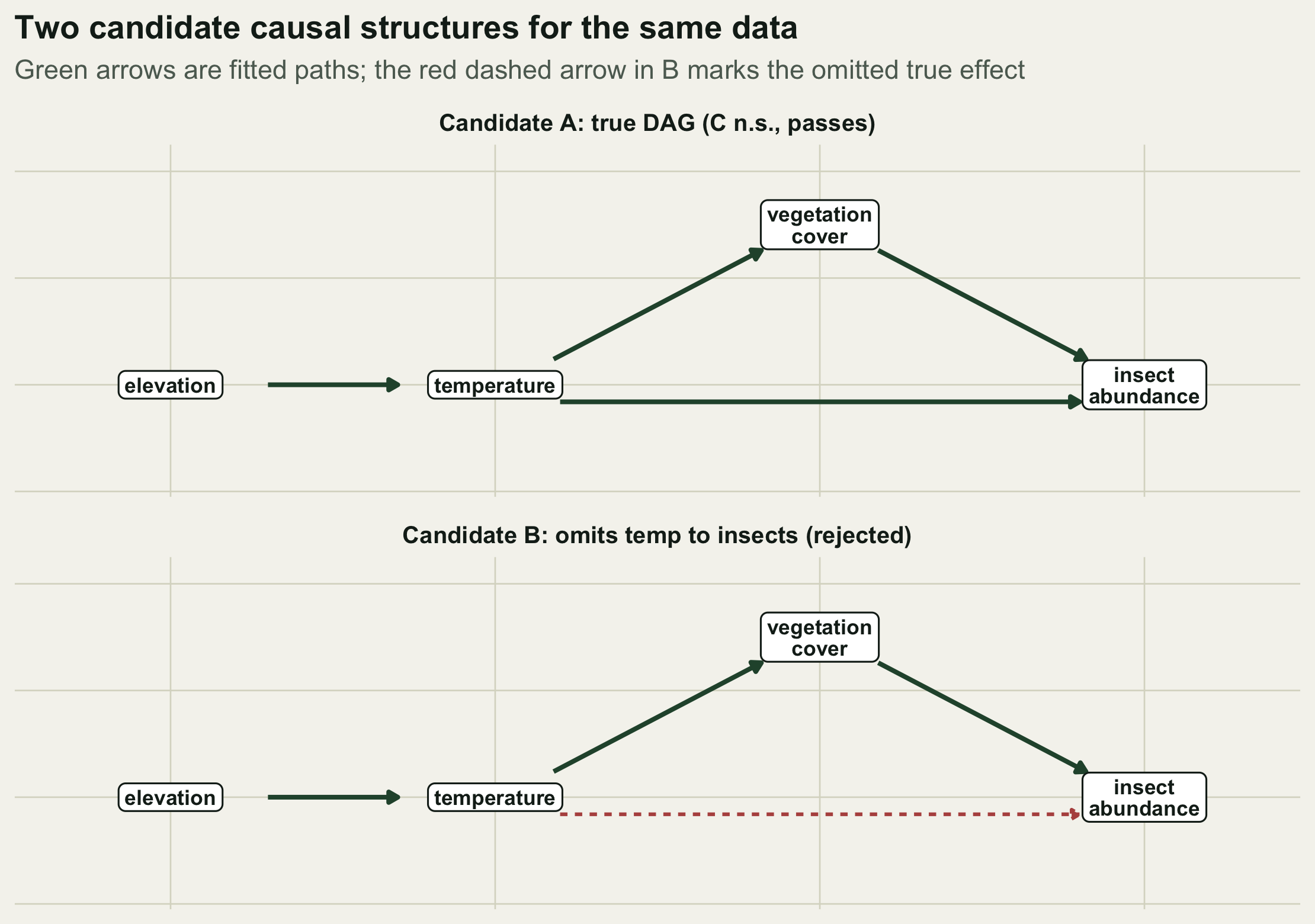
A missing edge, and where the test finds it
Now suppose a colleague proposes a leaner graph that drops the direct temperature to insects arrow, claiming insects respond only to vegetation. That graph implies a different, larger basis set, because temperature and insects are now non-adjacent as well.
pB1 <- claim_p("veg", "elevation", "temp", "gaussian")                 # holds
pB2 <- claim_p("insects", "elevation", "veg", "poisson")               # violated
pB3 <- claim_p("insects", "temp", c("veg","elevation"), "poisson")     # violated
CB  <- fishersC(c(pB1, pB2, pB3))
The first claim still holds (p = 0.79), but the other two collapse. Conditioning insects on vegetation alone leaves a clear residual link to elevation (p = 0.004), and temperature remains associated with insects after conditioning on vegetation and elevation (p = \(2.3 \times 10^{-8}\)). Fisher’s C jumps to 46.7 on 6 degrees of freedom, with p = \(2.1 \times 10^{-8}\). The model is rejected, and the two failed claims both point at the same thing: the dropped temperature to insects edge. The test does not just say the model is wrong; it tells you which independence the data refuse to grant.
sci_pm <- function(x) {   # plotmath text for a x 10^b, one significant digit
  s <- formatC(x, format = "e", digits = 0)
  sprintf("%s %%*%% 10^%d", sub("e.*", "", s), as.integer(sub(".*e", "", s)))
}
cl <- rbind(
  data.frame(candidate = sprintf('"Candidate A (C = %.2f, df 4, p = %.2f)"', CA["C"], CA["p"]),
             claim = c("elev _||_ veg | temp","elev _||_ ins | veg,temp"), p = c(pA1,pA2)),
  data.frame(candidate = sprintf('bold(paste("Candidate B (C = %.1f, df 6, p = ", %s, ")"))',
                                 CB["C"], sci_pm(CB["p"])),
             claim = c("elev _||_ veg | temp","elev _||_ ins | veg","temp _||_ ins | veg,elev"),
             p = c(pB1,pB2,pB3)))
cl$nlp <- -log10(cl$p); cl$violated <- cl$p < 0.05

ggplot(cl, aes(reorder(claim, nlp), nlp, fill = violated)) +
  geom_hline(yintercept = -log10(0.05), colour = te$warm, linetype = "22", linewidth = 0.5) +
  geom_col(width = 0.6) +
  geom_text(aes(label = ifelse(p < 0.001, sprintf('paste("p=", %s)', sci_pm(p)),
                        ifelse(p < 0.01, sprintf('"p=%.3f"',p), sprintf('"p=%.2f"',p)))),
            parse = TRUE, hjust = -0.08, size = 2.9, colour = te$body) +
  coord_flip(clip = "off") +
  facet_wrap(~candidate, ncol = 1, scales = "free_y", labeller = label_parsed) +
  scale_fill_manual(values = c(`FALSE` = te$sage, `TRUE` = te$warm),
                    labels = c("holds","violated (p < 0.05)"), name = NULL) +
  scale_y_continuous(expand = expansion(mult = c(0, 0.28))) +
  labs(title = "Every claim in the basis set, tested",
       subtitle = "Dashed line at p = 0.05; both violated claims in B involve the omitted edge",
       x = NULL, y = "-log10(p) of the tested absent path") +
  theme_te(12) + theme(legend.position = "top")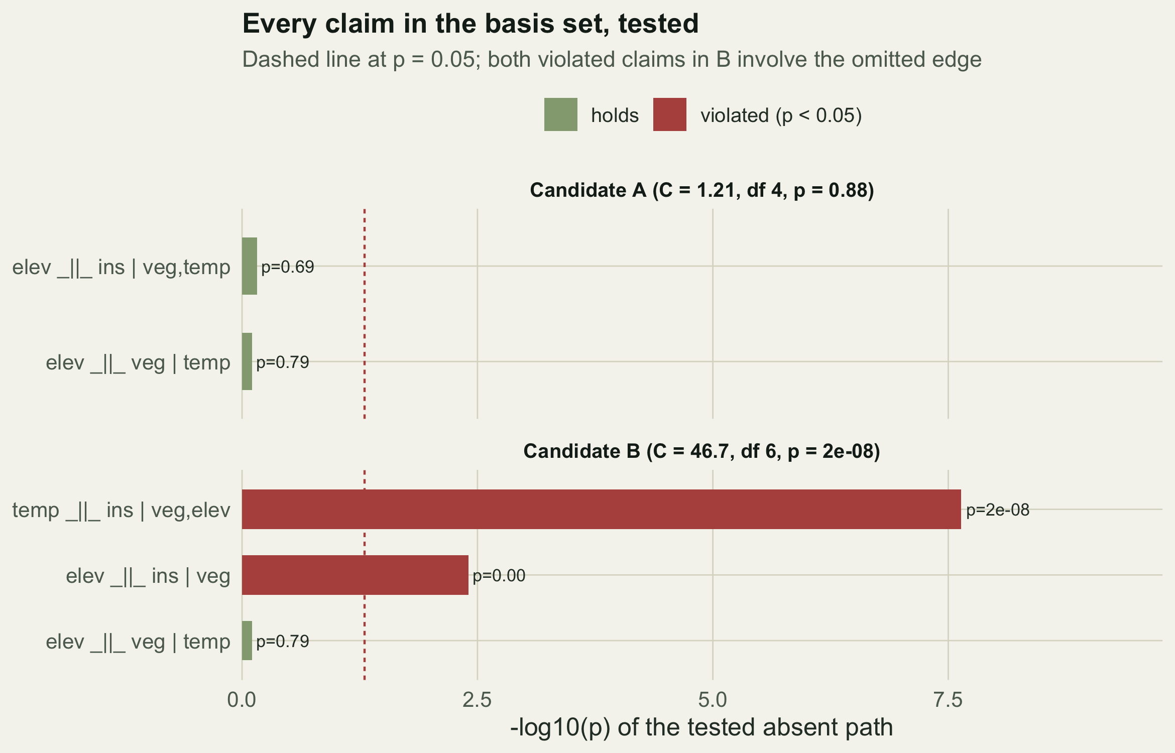
Comparing whole graphs with AIC
The d-separation statistic also supports model selection. Shipley (2013) defines an information criterion for a path model as its Fisher C plus twice the number of free path coefficients, AIC = C + 2K, which lets you rank non-nested graphs on the same footing.
KA <- 4; KB <- 3            # B estimates one fewer path
AICA <- unname(CA["C"] + 2 * KA)
AICB <- unname(CB["C"] + 2 * KB)
dAIC <- AICB - AICA
The true graph scores AIC = 9.2 against 52.7 for the leaner one, a difference of 43.5 in its favour. The extra path is not overfitting; it is a real effect, and both the significance test and the information criterion agree it belongs.
What d-separation does and does not test
Two limits are worth stating plainly. The test examines the absent arrows, the claims in the basis set; it never questions the arrows you did draw, nor their direction. A model can pass while its arrows point the wrong way, because reversing an arrow can leave the same set of implied independences. Separating those cases needs external knowledge or experiments, and it is the subject of the final post in this series. The test also assumes your conditioning sets capture the real confounders; an unmeasured common cause can make a wrong graph pass, or a right one fail, without any hint from the p-values.
Within those limits, the d-separation test is the natural companion to piecewise estimation. It gives a single, distribution-free verdict on a whole causal structure, and when that verdict is negative it hands you the specific independences to reconsider, which is a far more useful diagnosis than a lone rejection.
References
Lefcheck JS 2016 Methods in Ecology and Evolution 7(5):573-579 (10.1111/2041-210X.12512)
Shipley B 2000 Structural Equation Modeling 7(2):206-218 (10.1207/S15328007SEM0702_4)
Shipley B 2009 Ecology 90(2):363-368 (10.1890/08-1034.1)
Shipley B 2013 Ecology 94(3):560-564 (10.1890/12-0976.1)
Shipley B, Douma JC 2020 Ecology 101(3):e02960 (10.1002/ecy.2960)