Checking a structural equation model

Check a piecewise SEM in base R: calibrate Fisher’s C with a parametric bootstrap, and see why Markov-equivalent graphs fit identically and cannot orient the arrows.

Every model check answers two separate questions, and a structural equation model makes both unusually sharp. The first is whether the yardstick is trustworthy: the d-separation test judges a whole graph by comparing Fisher’s C against a chi-squared distribution, but that reference is asymptotic, so in a finite sample it may be the wrong ruler. The second, and deeper, question is what a passing test actually establishes. It is tempting to read a non-significant C as evidence that the arrows point the way you drew them. They do not follow. This closing post in the series checks both. A parametric bootstrap settles the first by simulating the reference distribution directly. A demonstration of Markov equivalence settles the second, and the answer is humbling: a model can pass while its arrows run backwards.

Is the chi-squared reference trustworthy here?

Recall from the d-separation post that Fisher’s C combines the p-values of a graph’s implied independences, and that C follows a chi-squared distribution with twice as many degrees of freedom as there are claims. That distribution is exact only in the limit of large samples. With forty observations it is an approximation, and the honest move is to check it rather than trust it. A parametric bootstrap does exactly that: fit the model, treat the fitted coefficients as truth, simulate many datasets from them, and recompute C each time. The spread of those values is the reference distribution the test actually faces.

library(ggplot2)

te <- list(paper="#f5f4ee", card="#ffffff", ink="#16241d", body="#2c3a31",
           forest="#275139", label="#46604a", sage="#93a87f", line="#dad9ca",
           muted="#5d6b61", warm="#b5534e", gold="#cda23f")

theme_te <- function(base_size = 12) {
  theme_minimal(base_size = base_size) +
    theme(plot.background  = element_rect(fill = te$paper, colour = NA),
          panel.background = element_rect(fill = te$paper, colour = NA),
          panel.grid.major = element_line(colour = te$line, linewidth = 0.3),
          panel.grid.minor = element_blank(),
          axis.text  = element_text(colour = te$muted, size = base_size * 0.85),
          axis.title = element_text(colour = te$body),
          plot.title = element_text(colour = te$ink, face = "bold", size = base_size * 1.1),
          plot.subtitle = element_text(colour = te$muted, size = base_size * 0.9),
          strip.text = element_text(colour = te$ink, face = "bold"))
}

claim_p <- function(resp, pred, cond, data) {
  f <- as.formula(paste(resp, "~", paste(c(pred, cond), collapse = " + ")))
  summary(lm(f, data = data))$coefficients[pred, "Pr(>|t|)"]
}
fishersC <- function(ps) {
  C <- -2 * sum(log(ps)); df <- 2 * length(ps)
  c(C = C, df = df, p = pchisq(C, df, lower.tail = FALSE))
}

knitr::opts_chunk$set(fig.align = "center", dev = "png", dpi = 150)

set.seed(158)
n <- 40
elevation <- rnorm(n)
temp <- -0.70 * elevation + sqrt(1 - 0.7^2) * rnorm(n)
veg  <-  0.60 * temp      + sqrt(1 - 0.6^2) * rnorm(n)
insects <- 0.55 * veg + 0.45 * temp + rnorm(n)
d0 <- data.frame(elevation, temp, veg, insects)

## correct graph: elev -> temp -> veg -> insects, temp -> insects; basis set has 2 claims
Cc <- fishersC(c(claim_p("veg", "elevation", "temp", d0),
                 claim_p("insects", "elevation", c("veg","temp"), d0)))
## misspecified graph: drop temp -> insects; basis set grows to 3 claims
Cm <- fishersC(c(claim_p("veg", "elevation", "temp", d0),
                 claim_p("insects", "elevation", "veg", d0),
                 claim_p("insects", "temp", c("veg","elevation"), d0)))

The correct graph gives C = 6.84 on 4 degrees of freedom, with an asymptotic p of 0.145. The misspecified graph, which drops the real temperature to insects arrow, gives C = 21.94 on 6 degrees of freedom (asymptotic p = 0.0012). Now the bootstrap check. Fitting the correct model and simulating from it gives a null distribution for C that we can compare against both the correct and the misspecified observed values.

f_temp <- lm(temp ~ elevation, d0); f_veg <- lm(veg ~ temp, d0)
f_ins  <- lm(insects ~ veg + temp, d0)
s_temp <- summary(f_temp)$sigma; s_veg <- summary(f_veg)$sigma; s_ins <- summary(f_ins)$sigma

simC <- function() {
  el <- rnorm(n, 0, sd(elevation))
  tp <- coef(f_temp)[1] + coef(f_temp)[2]*el + rnorm(n, 0, s_temp)
  vg <- coef(f_veg)[1]  + coef(f_veg)[2]*tp  + rnorm(n, 0, s_veg)
  is <- coef(f_ins)[1]  + coef(f_ins)[2]*vg  + coef(f_ins)[3]*tp + rnorm(n, 0, s_ins)
  dd <- data.frame(elevation = el, temp = tp, veg = vg, insects = is)
  unname(fishersC(c(claim_p("veg","elevation","temp", dd),
                    claim_p("insects","elevation",c("veg","temp"), dd)))["C"])
}
set.seed(9158)
B <- 3000
boot_C <- replicate(B, simC())
p_boot_correct <- mean(boot_C >= Cc["C"])
q95_boot <- unname(quantile(boot_C, 0.95)); q95_chi <- qchisq(0.95, Cc["df"])

The bootstrap null closely tracks the chi-squared curve: its 95th percentile is 9.66 against the chi-squared value of 9.49, and its mean is 4.04 against the chi-squared mean of 4. So at this sample size the asymptotic reference is safe to use, which is a conclusion worth having rather than assuming. Against that null the correct model is unremarkable (bootstrap p = 0.15, so it is not rejected), while the misspecified C of 21.9 sits far out in the tail. The bootstrap is cheap insurance; it earns its cost when a response is a count or the sample is smaller, where the chi-squared approximation can drift and this simulated reference is the one to believe.

xs  <- seq(0, max(quantile(boot_C, 0.999), Cc["C"]) + 1, length.out = 400)
chi <- data.frame(x = xs, dens = dchisq(xs, Cc["df"]))
ggplot() +
  geom_histogram(data = data.frame(boot_C), aes(boot_C, after_stat(density)),
                 bins = 45, fill = te$sage, colour = NA, alpha = 0.85) +
  geom_line(data = chi, aes(x, dens), colour = te$muted, linewidth = 0.9, linetype = "22") +
  geom_vline(xintercept = Cc["C"], colour = te$forest, linewidth = 1.0) +
  annotate("text", x = Cc["C"], y = max(chi$dens) * 0.92,
           label = sprintf("correct model\nC = %.2f\nbootstrap p = %.2f", Cc["C"], p_boot_correct),
           colour = te$forest, size = 3.0, hjust = -0.08, lineheight = 0.9) +
  annotate("segment", x = quantile(boot_C, 0.95), xend = quantile(boot_C, 0.995),
           y = 0.02, yend = 0.02, colour = te$warm, linewidth = 0.5,
           arrow = arrow(length = unit(0.12, "cm"))) +
  annotate("text", x = quantile(boot_C, 0.90), y = 0.055,
           label = sprintf("misspecified model C = %.1f\nfar in the tail", Cm["C"]),
           colour = te$warm, size = 2.9, hjust = 0.1, lineheight = 0.9) +
  labs(title = "Checking the yardstick: bootstrap the null of Fisher's C",
       subtitle = sprintf("The bootstrap null (grey) tracks chi-squared(%d) (dashed): 95th percentile %.2f vs %.2f",
                          Cc["df"], q95_boot, q95_chi),
       x = "Fisher's C under the fitted correct model", y = "density") +
  theme_te(12)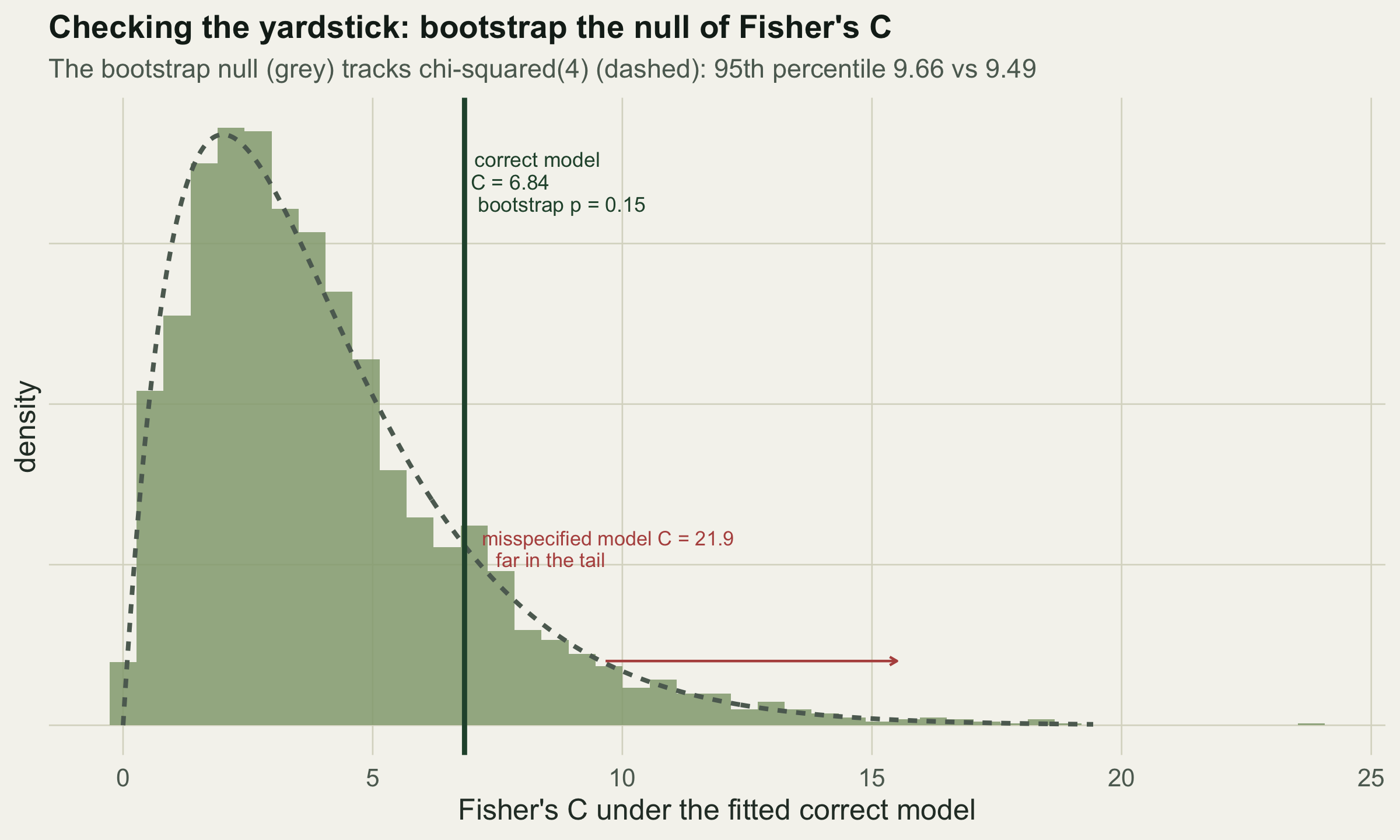 + theme(axis.text.y = element_blank())

Figure 1

What a passing test cannot tell you

Suppose the check passes. The graph is compatible with the data; the yardstick is sound. It is natural to feel the arrows have been vindicated. They have not, and the reason is structural. A directed graph implies a set of conditional independences, and the d-separation test examines exactly that set. Different graphs can imply the same set. When they do, they are indistinguishable to any test built on conditional independence, no matter how much data you collect. This is Markov equivalence (Verma and Pearl 1990), and it puts a hard ceiling on what observational fitting can recover.

The plainest case has three variables. Generate data where a driver acts on a response through a mediator, a simple chain.

set.seed(2158)
n2 <- 120
X <- rnorm(n2)
M <- 0.60 * X + sqrt(1 - 0.6^2) * rnorm(n2)
Y <- 0.60 * M + sqrt(1 - 0.6^2) * rnorm(n2)
d2 <- data.frame(X, M, Y)

Three different graphs all imply the single independence that X and Y are conditionally independent given M: the forward chain X to M to Y, the same chain reversed Y to M to X, and the common-cause fork where M drives both X and Y. Each is tested by the partial association of X and Y after conditioning on M, and partial association is symmetric, so all three return the identical result.

p_chain_fwd <- claim_p("Y", "X", "M", d2)     # X _||_ Y | M, framed forward
p_chain_bwd <- claim_p("X", "Y", "M", d2)     # X _||_ Y | M, framed backward
C_equiv <- fishersC(p_chain_fwd)

## the collider X -> M <- Y is a different class: it implies X _||_ Y marginally
p_marginal <- summary(lm(Y ~ X, d2))$coefficients["X", "Pr(>|t|)"]
C_collider <- fishersC(p_marginal)

The tested independence holds (p = 0.772), and framing it forward or backward gives the same p to the last digit, so all three equivalent graphs score an identical C = 0.52 and pass. No feature of the data prefers one over another. The chain that says nitrogen drives biomass, the chain that says biomass drives nitrogen, and the fork that says a third variable drives both are, to this test, the same model.

The collider is the instructive exception. A graph in which X and Y both point into M implies that X and Y are independent marginally, without conditioning on M. In chain data they are plainly associated through M, so that claim fails: the collider gives C = 20.9 with p = 2.9^{-5}, and is rejected. The test can therefore rule out a graph from a different equivalence class, but it is powerless to orient the arrows within one.

nx <- data.frame(node = c("X","M","Y"), x = c(0,1,2), y = c(0,1,0))
edef <- list(
  "X -> M -> Y  (chain)"          = list(c("X","M"), c("M","Y")),
  "Y -> M -> X  (chain reversed)" = list(c("Y","M"), c("M","X")),
  "X <- M -> Y  (common cause)"   = list(c("M","X"), c("M","Y")),
  "X -> M <- Y  (collider)"       = list(c("X","M"), c("Y","M")))
plab <- c("X -> M -> Y  (chain)"          = sprintf("C = %.2f, p = %.2f  (passes)", C_equiv["C"], C_equiv["p"]),
          "Y -> M -> X  (chain reversed)" = sprintf("C = %.2f, p = %.2f  (passes)", C_equiv["C"], C_equiv["p"]),
          "X <- M -> Y  (common cause)"   = sprintf("C = %.2f, p = %.2f  (passes)", C_equiv["C"], C_equiv["p"]),
          "X -> M <- Y  (collider)"       = sprintf("C = %.1f, p < 0.001  (rejected)", C_collider["C"]))
mk_edges <- function(pairs, panel) do.call(rbind, lapply(pairs, function(pr) {
  a <- nx[nx$node == pr[1], ]; b <- nx[nx$node == pr[2], ]
  dx <- b$x - a$x; dy <- b$y - a$y; L <- sqrt(dx^2 + dy^2)
  data.frame(x = a$x + 0.22*dx/L, y = a$y + 0.22*dy/L,
             xend = b$x - 0.22*dx/L, yend = b$y - 0.22*dy/L, panel = panel)
}))
edges <- do.call(rbind, Map(mk_edges, edef, names(edef)))
nodes <- do.call(rbind, lapply(names(edef), function(p) cbind(nx, panel = p)))
labs  <- data.frame(panel = names(plab), lab = unname(plab),
                    col = ifelse(grepl("rejected", plab), te$warm, te$forest))
for (df in c("edges","nodes","labs"))
  assign(df, within(get(df), panel <- factor(panel, levels = names(edef))))

ggplot() +
  geom_segment(data = edges, aes(x, y, xend = xend, yend = yend), colour = te$forest,
               linewidth = 0.9, arrow = arrow(length = unit(0.16, "cm"), type = "closed")) +
  geom_label(data = nodes, aes(x, y, label = node), fill = te$card, colour = te$ink,
             label.size = 0.4, label.r = unit(0.14, "cm"), size = 4.2, fontface = "bold") +
  geom_text(data = labs, aes(x = 1, y = -0.55, label = lab), colour = labs$col, size = 3.1) +
  facet_wrap(~panel, ncol = 2) +
  coord_cartesian(xlim = c(-0.35, 2.35), ylim = c(-0.8, 1.35), clip = "off") +
  labs(title = "The test reads the equivalence class, not the arrows",
       subtitle = "Data from X to M to Y: the three equivalent graphs fit identically; only the collider is a different class") +
  theme_te(12) +
  theme(axis.text = element_blank(), axis.title = element_blank(), panel.grid = element_blank())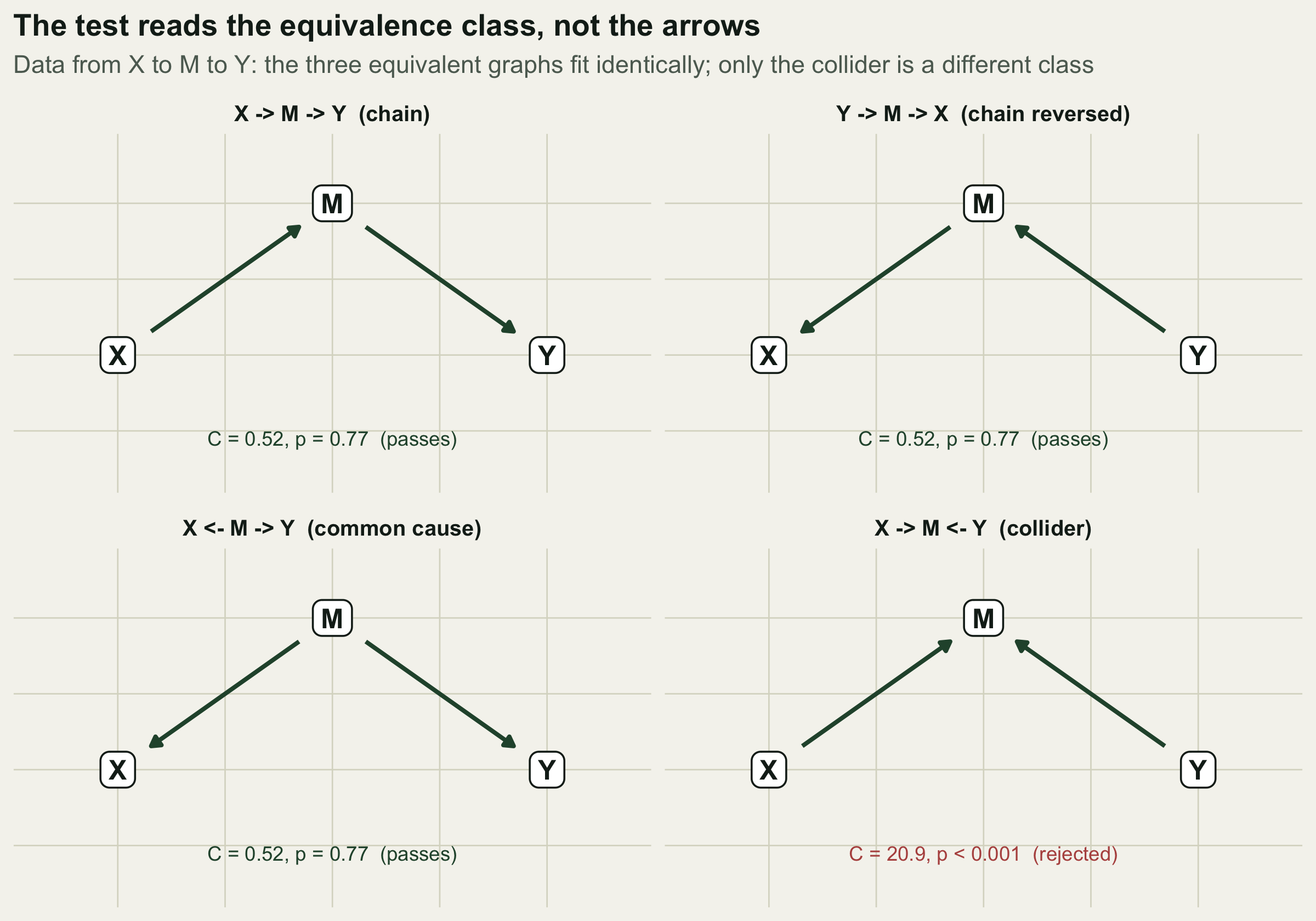

Warning: The `label.size` argument of `geom_label()` is deprecated as of ggplot2 3.5.0.
ℹ Please use the `linewidth` argument instead.

Figure 2

What checking buys, and what it does not

A d-separation test does real work. It can reject a structure whose implied independences the data refuse, as it rejected the collider and, earlier, the graph missing a true edge. It can be made honest about its own reference distribution with a parametric bootstrap, so a borderline p is trusted for the right reason. Those are worth doing on every fitted model.

What it cannot do is supply the direction of causation. Within an equivalence class the arrows are free, and an unmeasured common cause can let a wrong graph pass while a right one is rejected, with no signal in any p-value. That direction has to come from outside the data: a manipulation, a known time order, a mechanism that makes one direction impossible. This is the quiet assumption underneath the whole series. The path coefficients, the d-separation test, and the bootstrapped indirect effects are all conditional on the graph, and the graph is where the causal commitments live. The statistics will tell you whether a structure is contradicted; they will not tell you it is true. Keeping those two apart is most of what it means to use structural equation models well.

References

Grace, J. B., Anderson, T. M., Olff, H. and Scheiner, S. M. (2010). On the specification of structural equation models for ecological systems. Ecological Monographs 80(1): 67-87. DOI: 10.1890/09-0464.1

Shipley, B. (2000). A new inferential test for path models based on directed acyclic graphs. Structural Equation Modeling 7(2): 206-218. DOI: 10.1207/S15328007SEM0702_4

Shipley, B. (2013). The AIC model selection method applied to path analytic models compared using a d-separation test. Ecology 94(3): 560-564. DOI: 10.1890/12-0976.1

Shipley, B. and Douma, J. C. (2020). Generalized AIC and chi-squared statistics for path models consistent with directed acyclic graphs. Ecology 101(3): e02960. DOI: 10.1002/ecy.2960

Verma, T. and Pearl, J. (1990). Equivalence and synthesis of causal models. In Proceedings of the Sixth Conference on Uncertainty in Artificial Intelligence, 255-268. Elsevier Science.

Related tutorials

• Path analysis: direct and indirect effects
• Piecewise SEM and d-separation
• Checking causal assumptions
• checking-a-state-space-model

References

Grace JB, Anderson TM, Olff H, Scheiner SM 2010 Ecological Monographs 80(1):67-87 (10.1890/09-0464.1)
Shipley B 2000 Structural Equation Modeling 7(2):206-218 (10.1207/S15328007SEM0702_4)
Shipley B 2013 Ecology 94(3):560-564 (10.1890/12-0976.1)
Shipley B, Douma JC 2020 Ecology 101(3):e02960 (10.1002/ecy.2960)
Verma T, Pearl J 1990 Proceedings of the Sixth Conference on Uncertainty in Artificial Intelligence, 255-268. Elsevier Science