---
title: "Checking causal assumptions"
description: "You cannot prove there is no hidden confounder, but you can check. Negative controls and the robustness value put honest bounds on an untestable premise."
date: "2026-05-25 14:00"
categories: [causal inference, R, ecology tutorial, regression, sensitivity analysis]
image: thumbnail.png
image-alt: "A single coefficient plot with two estimates and their intervals: a dark green primary effect near 1.2, well above the dashed truth line at 0.5, and a red negative control near 0.7, far above the zero it should sit at."
---
The three previous posts all leaned on the same promise: that the causal graph is right, that the backdoor set is complete, that no unmeasured variable is quietly confounding the estimate. That promise is not testable. The data fix the associations, never the arrows, so no regression output can certify that adjustment closed every backdoor. What you can do is check the promise indirectly: look for footprints that hidden confounding would leave, and quantify how strong it would have to be to matter. Neither check confirms the premise. Both make it harder to fool yourself, which is the honest goal.
## A negative control leaves a footprint
A negative-control outcome is a placebo response: something the treatment cannot plausibly cause, but that shares the treatment's confounders. If the estimate is clean, the treatment should show no association with the placebo. If it does, a backdoor is open, because only confounding could link a treatment to an outcome it does not affect. Take a treatment with a true effect on the real outcome, and compare an unconfounded world with one where a hidden variable drives the treatment, the outcome, and the placebo alike.
```{r}
#| label: setup
#| code-fold: true
#| code-summary: "Setup: packages, colours and plot theme"
#| results: hide
#| message: false
#| warning: false
library(ggplot2)
paper <- "#f5f4ee"; ink <- "#16241d"; body <- "#2c3a31"
forest <- "#275139"; faint <- "#5d6b61"; line_col <- "#dad9ca"
red <- "#b5534e"; green <- "#2f8f63"; gold <- "#cda23f"
theme_te <- function(base_size = 12){
  theme_minimal(base_size = base_size) +
    theme(plot.background = element_rect(fill = paper, colour = NA),
          panel.background = element_rect(fill = paper, colour = NA),
          panel.grid.minor = element_blank(),
          panel.grid.major = element_line(colour = line_col, linewidth = 0.3),
          text = element_text(colour = body),
          plot.title = element_text(colour = ink, face = "bold"),
          plot.subtitle = element_text(colour = faint),
          axis.text = element_text(colour = faint),
          strip.text = element_text(colour = ink, face = "bold"),
          legend.position = "top")
}
```
```{r}
#| label: negative-control
true_eff <- 0.5; n <- 400
set.seed(162)                                  # Scenario A: unconfounded
XA <- rnorm(n)
YA <- true_eff * XA + rnorm(n, 0, 1)           # only X drives Y
NA_ <- rnorm(n, 0, 1)                            # placebo: nothing links it to X
mA  <- lm(YA ~ XA);  ncA <- lm(NA_ ~ XA)
sA  <- coef(mA)["XA"];  ciA  <- confint(mA)["XA", ]
ncA_c <- coef(ncA)["XA"]; ci_ncA <- confint(ncA)["XA", ]

set.seed(1620)                                  # Scenario B: an unmeasured confounder U
U  <- rnorm(n)
XB <- 0.9 * U + rnorm(n, 0, 0.6)
YB <- true_eff * XB + 0.9 * U + rnorm(n, 0, 1)  # true effect still 0.5, plus confounding
NB <- 0.9 * U + rnorm(n, 0, 1)                   # placebo: driven by U, NOT by X
mB  <- lm(YB ~ XB);  ncB <- lm(NB ~ XB)
sB  <- coef(mB)["XB"];  ciB  <- confint(mB)["XB", ]
ncB_c <- coef(ncB)["XB"]; ci_ncB <- confint(ncB)["XB", ]
corrected_B <- sB - ncB_c                        # subtract the bias the control reveals
```
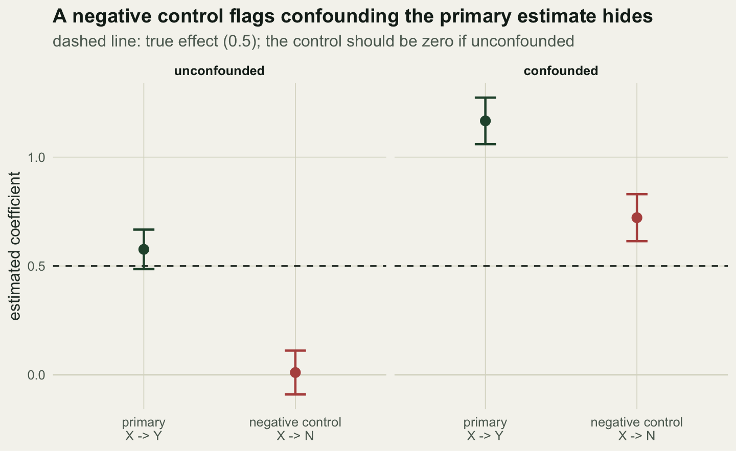
In the unconfounded world the primary estimate is `r round(sA, 3)`, interval [`r round(ciA[1], 2)`, `r round(ciA[2], 2)`], near the true `r true_eff`, and the negative control sits at `r round(ncA_c, 3)`, interval [`r round(ci_ncA[1], 2)`, `r round(ci_ncA[2], 2)`], astride zero. No alarm. In the confounded world the primary estimate inflates to `r round(sB, 3)`, interval [`r round(ciB[1], 2)`, `r round(ciB[2], 2)`], and the placebo, which the treatment cannot touch, comes back at `r round(ncB_c, 3)`, interval [`r round(ci_ncB[1], 2)`, `r round(ci_ncB[2], 2)`], firmly above zero. That non-null placebo is the footprint of an open backdoor, visible without ever measuring the confounder.
```{r}
#| label: fig-negative-control
#| fig-cap: "The primary estimate and a negative-control estimate in each world. The control (X to N) should sit at zero. When it does not, as in the confounded panel, it exposes confounding that the primary estimate silently absorbs."
#| fig-alt: "Two facets. Left, unconfounded: the primary point sits just above the dashed true-effect line with its interval covering it, the control point on zero. Right, confounded: the primary point sits well above the true effect and the control point well above zero."
#| fig-width: 7.5
#| fig-height: 4.6
f1 <- data.frame(
  scen = factor(rep(c("unconfounded", "confounded"), each = 2), levels = c("unconfounded", "confounded")),
  what = factor(rep(c("primary\nX -> Y", "negative control\nX -> N"), 2),
                levels = c("primary\nX -> Y", "negative control\nX -> N")),
  est = c(sA, ncA_c, sB, ncB_c),
  lo  = c(ciA[1], ci_ncA[1], ciB[1], ci_ncB[1]),
  hi  = c(ciA[2], ci_ncA[2], ciB[2], ci_ncB[2]))
ggplot(f1, aes(what, est, colour = what)) +
  geom_hline(yintercept = 0, colour = line_col, linewidth = 0.5) +
  geom_hline(yintercept = true_eff, linetype = "dashed", colour = ink) +
  geom_errorbar(aes(ymin = lo, ymax = hi), width = 0.14, linewidth = 0.8) +
  geom_point(size = 3) +
  facet_wrap(~scen) +
  scale_colour_manual(values = c("primary\nX -> Y" = forest, "negative control\nX -> N" = red), guide = "none") +
  labs(x = NULL, y = "estimated coefficient",
       title = "A negative control flags confounding the primary estimate hides",
       subtitle = "dashed line: true effect (0.5); the control should be zero if unconfounded") +
  theme_te()
```
Because the placebo carries the same confounding as the real outcome, its estimate is roughly the bias itself. Subtracting it, `r round(sB, 3)` minus `r round(ncB_c, 3)`, gives `r round(corrected_B, 3)`, back within reach of the true `r true_eff`. That calibration only works when the placebo shares the confounding structure of the outcome, an assumption you bring from [subject knowledge](../confounding-and-backdoor-adjustment/), not something the data confirm.
## How much confounding would it take?
The second check quantifies fragility. The robustness value of Cinelli and Hazlett asks: what share of the residual variance in both the treatment and the outcome would an unmeasured confounder need to explain to pull the estimate down to zero? It is computed from the coefficient's own t-statistic, so it needs no extra data, and it maps directly to a bias-adjusted estimate as the assumed confounding strength grows.
```{r}
#| label: robustness-value
rv_from_t <- function(tval, df, q = 1){          # Cinelli & Hazlett (2020)
  f <- q * abs(tval) / sqrt(df); 0.5 * (sqrt(f^4 + 4 * f^2) - f^2)
}
tA <- summary(mA)$coefficients["XA", "t value"]; rvA <- rv_from_t(tA, df.residual(mA))
tB <- summary(mB)$coefficients["XB", "t value"]; rvB <- rv_from_t(tB, df.residual(mB))
adj_curve <- function(est, se, df, r) sign(est) * (abs(est) - se * sqrt(df) * (r / sqrt(1 - r)))
seA <- summary(mA)$coefficients["XA", "Std. Error"]
seB <- summary(mB)$coefficients["XB", "Std. Error"]
```
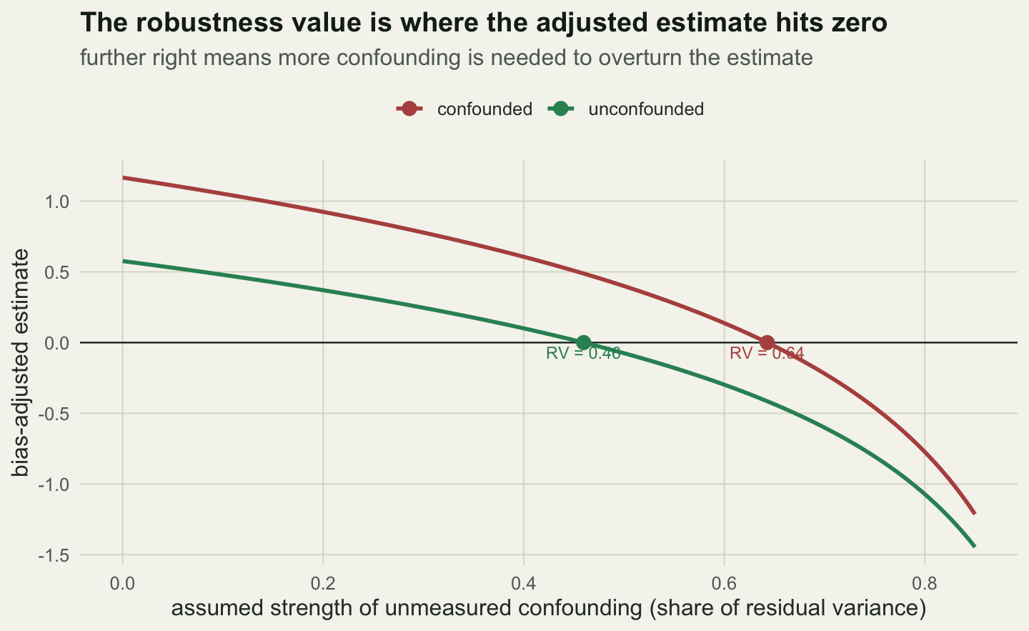
The unconfounded estimate has a robustness value of `r round(rvA, 3)`: a confounder would need to explain about `r round(100 * rvA, 0)`% of the leftover variance in both treatment and outcome to erase it. The confounded estimate returns `r round(rvB, 3)`, higher still. That is the catch worth sitting with. The confounded estimate is larger, so on paper it looks harder to overturn; the robustness value, read on its own, would call the biased result the safer of the two. The statistic measures how much confounding would be required, never how much is present. The negative control answers that second question, and here it has already fired.
```{r}
#| label: fig-robustness
#| fig-cap: "Bias-adjusted estimate as assumed confounding strength increases, for both worlds. Each curve reaches zero at its robustness value. The confounded curve crosses further right: paradoxically, its larger estimate would take more confounding to explain away, which is why the value cannot stand in for evidence about real confounding."
#| fig-alt: "Two downward curves against confounding strength on the x-axis. The green unconfounded curve reaches zero near 0.46; the red confounded curve reaches zero near 0.64, marked with their robustness values."
#| fig-width: 7.5
#| fig-height: 4.6
rgrid <- seq(0, 0.85, by = 0.005)
dfc <- rbind(
  data.frame(r = rgrid, adj = adj_curve(sA, seA, df.residual(mA), rgrid), scen = "unconfounded"),
  data.frame(r = rgrid, adj = adj_curve(sB, seB, df.residual(mB), rgrid), scen = "confounded"))
cross <- data.frame(scen = c("unconfounded", "confounded"), rv = c(rvA, rvB), y = 0,
                    lab = sprintf("RV = %.2f", c(rvA, rvB)))
ggplot(dfc, aes(r, adj, colour = scen)) +
  geom_hline(yintercept = 0, colour = ink, linewidth = 0.4) +
  geom_line(linewidth = 1) +
  geom_point(data = cross, aes(rv, y, colour = scen), size = 3, inherit.aes = FALSE) +
  geom_text(data = cross, aes(rv + 0.015, y + 0.12, label = lab, colour = scen), hjust = 0,
            size = 3.1, inherit.aes = FALSE, show.legend = FALSE) +
  scale_colour_manual(values = c("unconfounded" = green, "confounded" = red), name = NULL) +
  labs(x = "assumed strength of unmeasured confounding (share of residual variance)",
       y = "bias-adjusted estimate",
       title = "The robustness value is where the adjusted estimate hits zero",
       subtitle = "further right means more confounding is needed to overturn the estimate") +
  theme_te()
```
## The honest limit
These checks constrain the problem; they do not close it. A null negative control is reassuring only against confounders that would also disturb the placebo; a hidden variable that moves the outcome but spares the control leaves no footprint here. A large robustness value says an implausibly strong confounder would be needed, not that none exists, and as the confounded example shows, a large value can even accompany a badly biased estimate. Every one of these tools bounds the space of alternative explanations without singling out the truth, the same wall reached in [Markov-equivalent structures](../checking-a-structural-equation-model/): the data narrow what is possible and then stop. Causal claims from observational data rest on assumptions that checks can stress but not prove. Reporting a sensitivity analysis alongside the estimate, and being plain about which confounders it does and does not rule out, is what keeps the conclusion honest.
## References
Arif S, MacNeil MA 2022. Ecology Letters 25(8):1741-1745 (10.1111/ele.14033).
Arif S, MacNeil MA 2023. Ecological Monographs 93(1):e1554 (10.1002/ecm.1554).
Cinelli C, Hazlett C 2020. Journal of the Royal Statistical Society Series B 82(1):39-67 (10.1111/rssb.12348).
Lipsitch M, Tchetgen Tchetgen E, Cohen T 2010. Epidemiology 21(3):383-388 (10.1097/EDE.0b013e3181d61eeb).
VanderWeele TJ, Ding P 2017. Annals of Internal Medicine 167(4):268-274 (10.7326/M16-2607).
## Related tutorials
- [Confounding and backdoor adjustment](../confounding-and-backdoor-adjustment/)
- [Before-after-control-impact designs](../before-after-control-impact/)
- [Sensitivity to unmeasured confounding](../sensitivity-to-unmeasured-confounding/)
- [Transporting an effect to a new region](../transporting-an-effect-to-a-new-region/)