---
title: "Before-after-control-impact designs"
description: "A before-after contrast confounds the impact with a trend and a control-impact contrast with a site difference: the BACI interaction differences both out in R."
date: "2026-05-25 13:00"
categories: [causal inference, R, ecology tutorial, experimental design, regression]
image: thumbnail.png
image-alt: "An interaction plot: a control line rising from before to after, an impact line starting higher and dropping, and a dashed counterfactual showing the gap that is the impact."
---
A disturbance hits one site: an effluent outfall, a storm, a restoration cut. You sampled the site before and after, and you sampled a nearby control. The obvious summaries both mislead. Compare the impact site before and after, and you have folded in whatever happened to the whole region between the two visits, a wet year, a good recruitment pulse. Compare the impact and control sites after the event, and you have folded in every way the two sites differed to begin with. Each single difference confounds the impact with something else, and the two can even point in opposite directions.
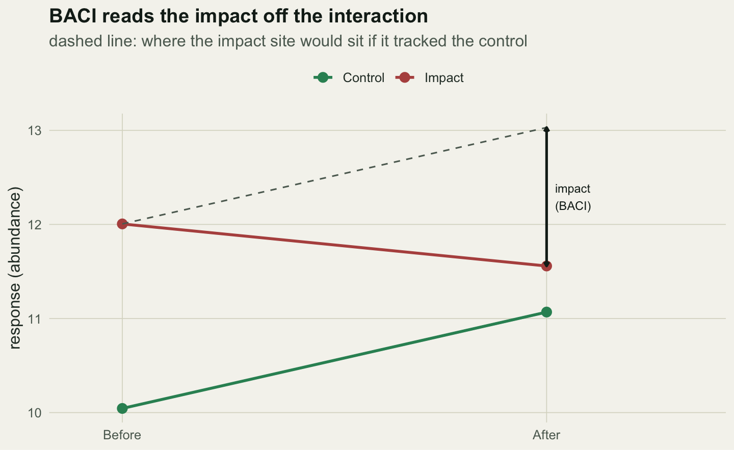
The before-after-control-impact (BACI) design fixes this by taking a difference of differences. The change at the impact site, minus the change at the control site, cancels the common regional trend (it hit both) and the fixed site gap (it was there before and after), leaving the impact. In a linear model this is exactly the site-by-time interaction. It works under one assumption, parallel trends, and that assumption is where the honesty lies.
## One impact, three answers
Let the response be an abundance. The control site starts at a baseline; the impact site starts higher for pre-existing reasons; a regional shift lifts both sites from the before period to the after period; and the disturbance lowers the impact site after the event. Only the last of these is what we want to measure.
```{r}
#| label: setup
#| code-fold: true
#| code-summary: "Setup: packages, colours and plot theme"
#| results: hide
#| message: false
#| warning: false
library(ggplot2)
paper <- "#f5f4ee"; ink <- "#16241d"; body <- "#2c3a31"
forest <- "#275139"; faint <- "#5d6b61"; line_col <- "#dad9ca"
red <- "#b5534e"; green <- "#2f8f63"
theme_te <- function(base_size = 12){
  theme_minimal(base_size = base_size) +
    theme(plot.background = element_rect(fill = paper, colour = NA),
          panel.background = element_rect(fill = paper, colour = NA),
          panel.grid.minor = element_blank(),
          panel.grid.major = element_line(colour = line_col, linewidth = 0.3),
          text = element_text(colour = body),
          plot.title = element_text(colour = ink, face = "bold"),
          plot.subtitle = element_text(colour = faint),
          axis.text = element_text(colour = faint),
          legend.position = "top")
}
```
```{r}
#| label: baci-fit
set.seed(161)
nrep  <- 40
mu0   <- 10     # control, before
site  <- 2      # impact site baseline higher (a pre-existing difference)
tim   <- 1      # common before -> after shift (e.g. a wet year)
delta <- -1.5   # TRUE impact: the disturbance lowers the impact site after
sdv   <- 1.5
mk <- function(mean, k) rnorm(k, mean, sdv)
CB <- mk(mu0, nrep); CA <- mk(mu0 + tim, nrep)
IB <- mk(mu0 + site, nrep); IA <- mk(mu0 + site + tim + delta, nrep)

dat <- data.frame(
  y = c(CB, CA, IB, IA),
  siteF = factor(rep(c("Control", "Impact"), each = 2 * nrep), levels = c("Control", "Impact")),
  timeF = factor(rep(rep(c("Before", "After"), each = nrep), 2), levels = c("Before", "After")))

mC <- c(mean(CB), mean(CA)); mI <- c(mean(IB), mean(IA))
ba_impact <- mI[2] - mI[1]      # before vs after, impact site only
ci_after  <- mI[2] - mC[2]      # impact vs control, after only
fit  <- lm(y ~ siteF * timeF, data = dat)
baci <- coef(fit)["siteFImpact:timeFAfter"]
baci_ci <- confint(fit)["siteFImpact:timeFAfter", ]
```
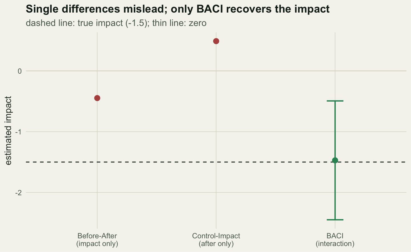
The four cell means come out at `r round(mC[1], 2)` and `r round(mC[2], 2)` for the control, `r round(mI[1], 2)` and `r round(mI[2], 2)` for the impact. Now read them three ways. The before-after change at the impact site is `r round(ba_impact, 3)`: a mild decline, because the regional lift partly masks the true drop. The impact-minus-control difference after the event is `r round(ci_after, 3)`, positive, because the impact site started higher and still sits above the control; taken alone it suggests the impact site is doing better, the opposite of the truth. The BACI interaction is `r round(baci, 3)`, interval [`r round(baci_ci[1], 2)`, `r round(baci_ci[2], 2)`], which lands on the true impact of `r delta`. The two simple contrasts are not just imprecise; one has the wrong sign.
```{r}
#| label: fig-interaction
#| fig-cap: "The BACI logic in one plot. The control changes from before to after; if the impact site had no disturbance it would change by the same amount (dashed counterfactual). The gap between that counterfactual and the observed impact-after mean is the BACI effect."
#| fig-alt: "An interaction plot with a green control line rising and a red impact line starting higher and falling. A grey dashed line extends the impact site parallel to the control; a double arrow marks the gap down to the observed point."
#| fig-width: 7.5
#| fig-height: 4.6
cf  <- data.frame(x = c(1, 2), y = c(mI[1], mI[1] + (mC[2] - mC[1])))
seg <- data.frame(x = 2, xend = 2, y = mI[1] + (mC[2] - mC[1]), yend = mI[2])
means <- data.frame(
  x = c(1, 2, 1, 2), y = c(mC[1], mC[2], mI[1], mI[2]),
  siteF = rep(c("Control", "Impact"), each = 2))
ggplot(means, aes(x, y, colour = siteF)) +
  geom_line(linewidth = 1) + geom_point(size = 3) +
  geom_line(data = cf, aes(x, y), colour = faint, linetype = "dashed", inherit.aes = FALSE) +
  geom_segment(data = seg, aes(x = x, xend = xend, y = y, yend = yend), colour = ink,
               linewidth = 0.9, arrow = arrow(length = unit(0.12, "cm"), ends = "both"),
               inherit.aes = FALSE) +
  annotate("text", x = 2.02, y = mean(c(mI[1] + (mC[2] - mC[1]), mI[2])),
           label = "impact\n(BACI)", hjust = 0, size = 3.1, colour = ink) +
  scale_colour_manual(values = c(Control = green, Impact = red), name = NULL) +
  scale_x_continuous(breaks = c(1, 2), labels = c("Before", "After"), limits = c(0.9, 2.35)) +
  labs(x = NULL, y = "response (abundance)",
       title = "BACI reads the impact off the interaction",
       subtitle = "dashed line: where the impact site would sit if it tracked the control") +
  theme_te()
```
The interaction is the whole point. A one-way comparison, before-after or control-impact, is a main effect, and a main effect cannot separate the disturbance from the backdrop. Isolating the disturbance means asking whether the impact site changed differently from the control, which is what the [interaction term](../interaction-terms-glm/) tests. This is also why a single control and a single impact site, sampled once each side of the event, is the design Stewart-Oaten and colleagues flagged as [pseudoreplication in time](../pseudoreplication-in-ecology/): the interaction rests on one site per condition, and real designs want several.
```{r}
#| label: fig-estimates
#| fig-cap: "The three estimates against the truth. Before-after understates the impact; control-impact reverses its sign; only the BACI interaction (with its 95% interval) recovers it."
#| fig-alt: "Three points against a dashed line at minus 1.5. The before-after point sits near zero, the control-impact point is positive, and the BACI point with an interval sits on the dashed line."
#| fig-width: 7.5
#| fig-height: 4.6
fig2 <- data.frame(
  contrast = factor(c("Before-After\n(impact only)", "Control-Impact\n(after only)", "BACI\n(interaction)"),
                    levels = c("Before-After\n(impact only)", "Control-Impact\n(after only)", "BACI\n(interaction)")),
  est = c(ba_impact, ci_after, baci),
  lo  = c(NA, NA, baci_ci[1]), hi = c(NA, NA, baci_ci[2]),
  kind = c("wrong", "wrong", "right"))
ggplot(fig2, aes(contrast, est, colour = kind)) +
  geom_hline(yintercept = delta, linetype = "dashed", colour = ink) +
  geom_hline(yintercept = 0, colour = line_col, linewidth = 0.4) +
  geom_errorbar(aes(ymin = lo, ymax = hi), width = 0.14, linewidth = 0.8, na.rm = TRUE) +
  geom_point(size = 3) +
  scale_colour_manual(values = c(right = green, wrong = red), guide = "none") +
  labs(x = NULL, y = "estimated impact",
       title = "Single differences mislead; only BACI recovers the impact",
       subtitle = "dashed line: true impact (-1.5); thin line: zero") +
  theme_te()
```
## What parallel trends buys, and what it costs
BACI removes the regional trend by borrowing the control's change as a stand-in for what the impact site would have done on its own. That substitution is the parallel-trends assumption: absent the disturbance, the two sites would have moved in step. When it holds, the interaction is the impact. When it fails, the interaction absorbs the divergence and reports it as impact, whether or not any impact occurred.
```{r}
#| label: parallel-trends
set.seed(1610)
diff_trend <- -1.2      # impact site drifting down for reasons unrelated to any impact
CB2 <- mk(mu0, nrep); CA2 <- mk(mu0 + tim, nrep)
IB2 <- mk(mu0 + site, nrep); IA2 <- mk(mu0 + site + tim + diff_trend, nrep)  # true impact = 0
dat2 <- data.frame(
  y = c(CB2, CA2, IB2, IA2),
  siteF = factor(rep(c("Control", "Impact"), each = 2 * nrep), levels = c("Control", "Impact")),
  timeF = factor(rep(rep(c("Before", "After"), each = nrep), 2), levels = c("Before", "After")))
fit2 <- lm(y ~ siteF * timeF, data = dat2)
baci2 <- coef(fit2)["siteFImpact:timeFAfter"]; baci2_ci <- confint(fit2)["siteFImpact:timeFAfter", ]
```
Here the disturbance does nothing; the impact site simply drifts downward on its own. BACI still returns `r round(baci2, 3)`, interval [`r round(baci2_ci[1], 2)`, `r round(baci2_ci[2], 2)`], excluding zero: a confident, entirely spurious impact, manufactured by a background trend the control did not share. A significant interaction is therefore necessary but not sufficient. It shows the sites diverged; it does not show the disturbance caused the divergence. Multiple controls, several before and after periods to gauge whether trends really run parallel, and explicit attention to [unmeasured drivers](../checking-causal-assumptions/) are what turn a BACI contrast into a defensible impact estimate. The design differences out the confounders it can see; parallel trends is the promise about the ones it cannot.
## References
Chevalier M, Russell JC, Knape J 2019. Ecological Applications 29(2):e01838 (10.1002/eap.1838).
Christie AP, Amano T, Martin PA, Shackelford GE, Simmons BI, Sutherland WJ 2019. Journal of Applied Ecology 56(12):2742-2754 (10.1111/1365-2664.13499).
Stewart-Oaten A, Murdoch WW, Parker KR 1986. Ecology 67(4):929-940 (10.2307/1939815).
Underwood AJ 1992. Journal of Experimental Marine Biology and Ecology 161(2):145-178 (10.1016/0022-0981(92)90094-Q).
Underwood AJ 1994. Ecological Applications 4(1):3-15 (10.2307/1942110).
## Related tutorials
- [Confounding and backdoor adjustment](../confounding-and-backdoor-adjustment/)
- [Checking causal assumptions](../checking-causal-assumptions/)
- [Baseline selection and the return to the mean](../baseline-selection-and-the-return-to-mean/)
- [Event-study difference-in-differences](../difference-in-differences-event-study/)