Path analysis: direct, indirect, and total effects

Split an ecological correlation into direct and indirect routes with lm in base R. Standardised path coefficients, the tracing rules, and why a bivariate slope misleads.

A single correlation coefficient tells you that two variables move together. It does not tell you why. In an ecological system, the association between a driver and a response usually runs along several routes at once: a direct effect, one or more indirect effects through intermediate variables, and sometimes a shared cause. Path analysis, the oldest branch of structural equation modelling, takes a hypothesised diagram of arrows and splits the observed correlation into those separate contributions. Sewall Wright worked this out for guinea-pig birth weights in the 1920s (Wright 1921, 1934), and the machinery is nothing more exotic than a few linear regressions read in the right order.

This post fits a small path model with lm, reads the path coefficients, and separates the direct from the indirect effect of a driver on a response. The recurring lesson: the bivariate slope you would report from a simple regression is an exact sum of the direct path and the indirect paths, so on its own it can hide a strong mediated effect, or even a direct effect that points the opposite way.

A three-variable system

The data are synthetic and illustrative. Picture a grassland where soil nitrogen raises plant biomass, biomass supports herbivores, and nitrogen also acts on herbivores directly (through tissue chemistry, say). The hypothesised diagram is nitrogen to biomass to herbivory, with an extra direct arrow from nitrogen to herbivory.

library(ggplot2)

te <- list(paper="#f5f4ee", card="#ffffff", ink="#16241d", body="#2c3a31",
           forest="#275139", label="#46604a", sage="#93a87f", line="#dad9ca",
           muted="#5d6b61", warm="#b5534e", gold="#cda23f")

theme_te <- function(base_size = 12) {
  theme_minimal(base_size = base_size) +
    theme(plot.background  = element_rect(fill = te$paper, colour = NA),
          panel.background = element_rect(fill = te$paper, colour = NA),
          panel.grid.major = element_line(colour = te$line, linewidth = 0.3),
          panel.grid.minor = element_blank(),
          axis.text  = element_text(colour = te$muted, size = base_size * 0.85),
          axis.title = element_text(colour = te$body),
          plot.title = element_text(colour = te$ink, face = "bold", size = base_size * 1.1),
          plot.subtitle = element_text(colour = te$muted, size = base_size * 0.9),
          strip.text = element_text(colour = te$ink, face = "bold"))
}

knitr::opts_chunk$set(fig.align = "center", dev = "png", dpi = 150)

set.seed(155)
n <- 150
nitrogen <- rnorm(n)
a_true <- 0.60
biomass <- a_true * nitrogen + sqrt(1 - a_true^2) * rnorm(n)
cprime_true <- 0.15
b_true <- 0.55
herbivory <- cprime_true * nitrogen + b_true * biomass + rnorm(n)

## standardise so that lm coefficients are standardised path coefficients
z <- function(x) (x - mean(x)) / sd(x)
nitrogen  <- z(nitrogen)
biomass   <- z(biomass)
herbivory <- z(herbivory)

Standardising every variable to mean zero and unit variance is a convenience: the slope from a regression on standardised variables is a standardised regression coefficient, which is exactly what a path coefficient is. It puts every arrow on the same scale (standard deviations of the response per standard deviation of the predictor), so the sizes are directly comparable. When absolute units matter more than comparability, you would keep the raw scale instead and interpret the paths in the original units.

Two regressions are the whole model

A path model with no feedback loops factorises into one regression per response variable, each conditioned on the arrows pointing into it. Biomass has one parent (nitrogen); herbivory has two (nitrogen and biomass). So the entire model is two lm calls.

m_bio <- lm(biomass ~ nitrogen)                # path a
m_her <- lm(herbivory ~ nitrogen + biomass)    # paths c' and b

a      <- unname(coef(m_bio)["nitrogen"])
cprime <- unname(coef(m_her)["nitrogen"])
b      <- unname(coef(m_her)["biomass"])

se_a  <- summary(m_bio)$coef["nitrogen", "Std. Error"]
se_cp <- summary(m_her)$coef["nitrogen", "Std. Error"]
se_b  <- summary(m_her)$coef["biomass",  "Std. Error"]
p_cp  <- summary(m_her)$coef["nitrogen", "Pr(>|t|)"]

The fitted paths are a = 0.584 (SE 0.067) for nitrogen to biomass, b = 0.576 (SE 0.079) for biomass to herbivory, and a direct path c’ = 0.087 (SE 0.079) for nitrogen to herbivory. Both a and b are strongly supported, but the direct path c’ has p = 0.27: on this evidence it is not distinguishable from zero.

Decomposing the correlation

The tracing rules give the total association between two variables as the sum over every valid path connecting them, and each path contributes the product of the coefficients along it. Here nitrogen reaches herbivory two ways: directly (c’) and through biomass (a times b). So

indirect <- a * b
total    <- cprime + indirect
prop_med <- indirect / total

## the exact identity: total equals the simple regression slope
m_naive   <- lm(herbivory ~ nitrogen)
total_reg <- unname(coef(m_naive)["nitrogen"])
r_xy      <- cor(nitrogen, herbivory)
gap       <- abs(total_reg - total)

The indirect effect is a times b = 0.336, the direct effect is 0.087, and their sum, the total effect, is 0.423. That total is not an approximation: it equals the slope from the naive regression lm(herbivory ~ nitrogen), which is 0.423, and equals the bivariate correlation 0.423 (the two coincide because both variables are standardised). The two numbers agree to 0, which is machine precision. The decomposition is an algebraic partition of the ordinary regression coefficient, not a separate model.

That identity is the point. A researcher who ran only the simple regression would report a slope of 0.423 and, without a diagram, would be tempted to read it as a direct effect of nitrogen on herbivory. The path model shows that 80% of that association travels through biomass, and that the direct link is essentially zero. The management implication is different: to move herbivory you would manage biomass, not nitrogen directly.

nodes <- data.frame(x = c(0,1,2), y = c(0,1,0),
                    lab = c("Soil\nnitrogen","Plant\nbiomass","Herbivory"))
edges <- data.frame(
  x1 = c(0.22, 1.20, 0.24), y1 = c(0.16, 0.84, 0),
  x2 = c(0.80, 1.78, 1.76), y2 = c(0.84, 0.16, 0),
  ltype = c("solid","solid","22"),
  col   = c(te$forest, te$forest, te$muted))
labs <- data.frame(
  x = c(0.5, 1.55, 1.0), y = c(0.62, 0.62, -0.16),
  lab = c(sprintf("a = %.2f", a), sprintf("b = %.2f", b),
          sprintf("c' = %.2f (ns)", cprime)),
  col = c(te$forest, te$forest, te$muted))

ggplot() +
  geom_segment(data = edges, aes(x = x1, y = y1, xend = x2, yend = y2),
               linetype = edges$ltype, colour = edges$col, linewidth = 0.9,
               arrow = arrow(length = unit(0.16, "cm"), type = "closed")) +
  geom_label(data = nodes, aes(x, y, label = lab), fill = te$card, colour = te$ink,
             label.size = 0.4, label.r = unit(0.12, "cm"), size = 3.6,
             lineheight = 0.9, fontface = "bold") +
  geom_text(data = labs, aes(x, y, label = lab), colour = labs$col, size = 3.2) +
  annotate("text", x = 1, y = 1.32,
           label = sprintf("naive bivariate r(nitrogen, herbivory) = %.2f", r_xy),
           colour = te$warm, size = 3.3) +
  coord_cartesian(xlim = c(-0.35, 2.35), ylim = c(-0.45, 1.5), clip = "off") +
  labs(title = "Two structural equations, three fitted paths",
       subtitle = "Standardised coefficients from lm(biomass ~ nitrogen) and lm(herbivory ~ nitrogen + biomass)") +
  theme_te(12) +
  theme(axis.text = element_blank(), axis.title = element_blank(),
        panel.grid = element_blank())

Warning: The `label.size` argument of `geom_label()` is deprecated as of ggplot2 3.5.0.
ℹ Please use the `linewidth` argument instead.

Figure 1

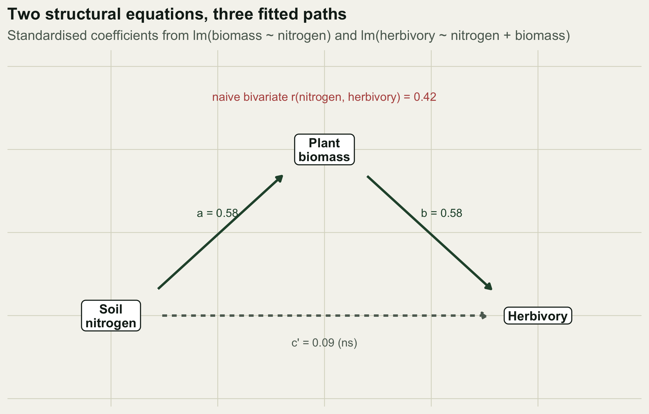
When the direct effect flips sign

The mostly-indirect case is common, but the more striking failure of a bare correlation is suppression: two real pathways of opposite sign that partly cancel. Here is a second system where nitrogen deters herbivores directly but promotes them through biomass.

set.seed(2155)
n2 <- 150
nit2 <- rnorm(n2)
a2t <- 0.70; cp2t <- -0.20; b2t <- 0.70
bio2 <- a2t * nit2 + sqrt(1 - a2t^2) * rnorm(n2)
her2 <- cp2t * nit2 + b2t * bio2 + rnorm(n2)
nit2 <- z(nit2); bio2 <- z(bio2); her2 <- z(her2)

a2  <- unname(coef(lm(bio2 ~ nit2))["nit2"])
mh2 <- lm(her2 ~ nit2 + bio2)
cp2 <- unname(coef(mh2)["nit2"]); b2 <- unname(coef(mh2)["bio2"])
ind2 <- a2 * b2; tot2 <- cp2 + ind2
r_xy2 <- cor(nit2, her2)

Now the bivariate correlation is 0.231, mildly positive: a simple analysis would conclude that nitrogen is weakly good for herbivores. The path model tells a sharper story. The indirect effect through biomass is 0.446 (positive and dominant), while the direct effect is -0.215 (negative). The sign of the direct path is the opposite of the sign of the correlation. No amount of staring at the raw scatter of nitrogen against herbivory would recover that; only the decomposition does.

mk <- function(direct, indirect, total, scn)
  data.frame(component = factor(c("direct (c')","indirect (a*b)","total"),
                                levels = c("direct (c')","indirect (a*b)","total")),
             value = c(direct, indirect, total), scenario = scn)
dd <- rbind(mk(cprime, indirect, total, "Main model: effect is mostly indirect"),
            mk(cp2,    ind2,     tot2,  "Suppression: direct effect flips sign"))
dd$fill <- ifelse(dd$component == "total", "total",
                  ifelse(dd$value < 0, "neg", "pos"))

ggplot(dd, aes(component, value, fill = fill)) +
  geom_hline(yintercept = 0, colour = te$muted, linewidth = 0.4) +
  geom_col(width = 0.62) +
  geom_text(aes(label = sprintf("%.2f", value),
                vjust = ifelse(value >= 0, -0.4, 1.3)),
            size = 3.1, colour = te$body) +
  facet_wrap(~scenario) +
  scale_fill_manual(values = c(pos = te$forest, neg = te$warm, total = te$sage),
                    guide = "none") +
  coord_cartesian(ylim = c(-0.32, 0.55)) +
  labs(title = "Total effect = direct + indirect",
       subtitle = "An exact partition of the OLS slope; it can hide a strong or oppositely signed direct path",
       x = NULL, y = "standardised effect of nitrogen on herbivory") +
  theme_te(12)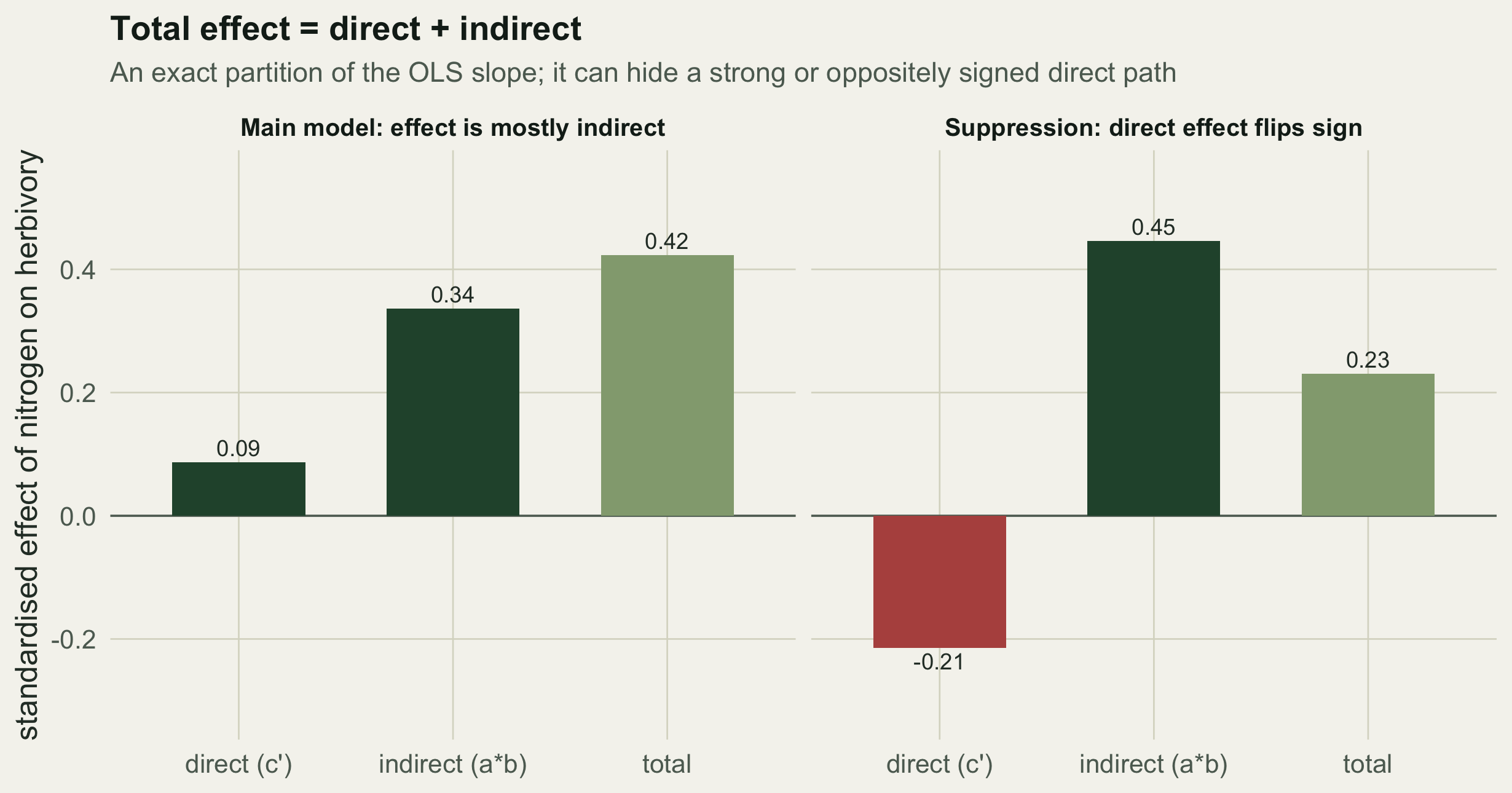

Figure 2

What the coefficients do and do not buy you

Two cautions keep path analysis honest. First, the arrows are an assumption. The regressions run happily on any diagram you hand them; they do not check that the diagram is correct, and the coefficients carry a causal reading only if the structure is right. Reversing an arrow or omitting a common cause changes the numbers without any warning from lm. Testing whether the assumed structure is even compatible with the data is a separate step, using the conditional independences the diagram implies; that is the subject of the next post on d-separation.

Second, standardised and unstandardised coefficients answer different questions. Standardised paths are comparable across variables on different measurement scales, which is why they suit a diagram; unstandardised paths keep biological units and transfer better across studies with different variances. Report whichever matches the question, and say which one it is.

With those caveats in mind, the decomposition is a genuinely useful habit. A correlation is a starting point, not a conclusion; splitting it into the routes a hypothesised diagram allows turns a single ambiguous number into a set of comparable, interpretable effects.

References

Grace, J. B. (2006). Structural Equation Modeling and Natural Systems. Cambridge University Press. ISBN 978-0-521-83409-3.

Grace, J. B. and Bollen, K. A. (2005). Interpreting the results from multiple regression and structural equation models. Bulletin of the Ecological Society of America 86(4): 283-295. DOI: 10.1890/0012-9623(2005)86[283:ITRFMR]2.0.CO;2

Grace, J. B., Anderson, T. M., Olff, H. and Scheiner, S. M. (2010). On the specification of structural equation models for ecological systems. Ecological Monographs 80(1): 67-87. DOI: 10.1890/09-0464.1

Wright, S. (1921). Correlation and causation. Journal of Agricultural Research 20: 557-585.

Wright, S. (1934). The method of path coefficients. The Annals of Mathematical Statistics 5(3): 161-215. DOI: 10.1214/aoms/1177732676

Related tutorials

• Piecewise SEM and d-separation
• Mediation and bootstrapped indirect effects
• collinearity-and-vif
• Confounding and backdoor adjustment