Mediation and bootstrapped indirect effects

Estimate a mediated effect in base R, then compare the Sobel normal interval with a bootstrap percentile interval. Why the product a times b needs resampling.

Mediation asks how much of a total effect passes through an intermediate variable. Split the total effect of a driver on a response into a direct part and an indirect part, and the indirect part is a product: the coefficient from driver to mediator (a) times the coefficient from mediator to response (b). Estimating a times b is easy. Putting a confidence interval on it is where the trouble starts, because the product of two normally distributed estimates is not itself normal. It is skewed, and the classical interval ignores that.

The classical route is the Sobel test: a standard error for a times b from the delta method, then a symmetric interval of the estimate plus or minus about two standard errors (Sobel 1982, Baron and Kenny 1986). It is quick and it is what many textbooks still teach. It also has a documented weakness (MacKinnon et al. 2002, 2004): because the sampling distribution of a times b is skewed, a symmetric normal interval sits in the wrong place and covers the true value less often than it claims. The fix is to stop assuming a shape and resample instead. This post fits a small mediation model in base R, builds both intervals by hand, and shows with a coverage simulation why the bootstrap earns its keep. The moral echoes the meta-analysis posts: a naive interval that assumes a convenient distribution reports more certainty than the data support.

A mediation model

The data are synthetic and illustrative: a driver x, a mediator m, and a response y, with a modest true indirect effect. The sample is deliberately small, because that is exactly the regime where the two methods part ways.

library(ggplot2)

te <- list(paper="#f5f4ee", card="#ffffff", ink="#16241d", body="#2c3a31",
           forest="#275139", label="#46604a", sage="#93a87f", line="#dad9ca",
           muted="#5d6b61", warm="#b5534e", gold="#cda23f")

theme_te <- function(base_size = 12) {
  theme_minimal(base_size = base_size) +
    theme(plot.background  = element_rect(fill = te$paper, colour = NA),
          panel.background = element_rect(fill = te$paper, colour = NA),
          panel.grid.major = element_line(colour = te$line, linewidth = 0.3),
          panel.grid.minor = element_blank(),
          axis.text  = element_text(colour = te$muted, size = base_size * 0.85),
          axis.title = element_text(colour = te$body),
          plot.title = element_text(colour = te$ink, face = "bold", size = base_size * 1.1),
          plot.subtitle = element_text(colour = te$muted, size = base_size * 0.9))
}

knitr::opts_chunk$set(fig.align = "center", dev = "png", dpi = 150)

A small helper fits the two regressions and returns the pieces we need, including the Sobel standard error from the delta method. Ordinary lm would do; the hand-coded least squares below is only so the same function can run thousands of times quickly in the simulation later.

ols <- function(X, y) {
  XtX <- crossprod(X); beta <- solve(XtX, crossprod(X, y))
  resid <- y - X %*% beta; s2 <- sum(resid^2) / (nrow(X) - ncol(X))
  list(beta = as.numeric(beta), se = sqrt(diag(solve(XtX)) * s2))
}
med_fit <- function(x, m, y) {
  e1 <- ols(cbind(1, x), m)              # m ~ x     gives a
  e2 <- ols(cbind(1, x, m), y)           # y ~ x + m gives c' and b
  a  <- unname(e1$beta[2]); se_a <- unname(e1$se[2])
  b  <- unname(e2$beta[3]); se_b <- unname(e2$se[3])
  ind <- a * b
  sob <- sqrt(b^2 * se_a^2 + a^2 * se_b^2)   # first-order Sobel (delta method)
  c(a = a, b = b, cprime = unname(e2$beta[2]), indirect = ind, sobelSE = sob)
}

a_t <- 0.35; b_t <- 0.35; cp_t <- 0.20
ind_true <- a_t * b_t
n <- 50

set.seed(157)
x <- rnorm(n)
m <- a_t * x + sqrt(1 - a_t^2) * rnorm(n)
y <- cp_t * x + b_t * m + rnorm(n)

fit <- med_fit(x, m, y)
prop_med <- unname(fit["indirect"] / (fit["cprime"] + fit["indirect"]))

In this sample the driver to mediator path is a = 0.25, the mediator to response path is b = 0.293, and the direct path is c’ = 0.148. The indirect effect is their product, a times b = 0.073, which is about 33% of the total effect. That point estimate is not in dispute between methods. The interval around it is.

The Sobel interval, and why its shape is wrong

The delta method gives a standard error for a times b, and the Sobel interval is the estimate plus or minus 1.96 of those standard errors.

sobelSE <- unname(fit["sobelSE"])
sob_lo  <- unname(fit["indirect"]) - 1.96 * sobelSE
sob_hi  <- unname(fit["indirect"]) + 1.96 * sobelSE

That returns a standard error of 0.053 and a 95% interval of [-0.031, 0.178], symmetric about the estimate by construction. The construction is the problem. A times b is a product of two roughly normal quantities, and such a product is skewed unless both coefficients are large relative to their errors. Forcing a symmetric interval onto a skewed quantity puts the bounds in the wrong places: usually too short on the long tail and too long on the short one.

The bootstrap makes no such assumption. Resample the rows with replacement, refit both equations, record a times b, and repeat; the spread of those values is the sampling distribution, read directly rather than approximated.

boot_ind <- function(x, m, y, B) {
  n <- length(x); out <- numeric(B)
  for (i in seq_len(B)) {
    idx <- sample.int(n, n, replace = TRUE)
    e1 <- ols(cbind(1, x[idx]), m[idx])
    e2 <- ols(cbind(1, x[idx], m[idx]), y[idx])
    out[i] <- e1$beta[2] * e2$beta[3]
  }
  out
}
set.seed(2157)
bd <- boot_ind(x, m, y, 5000)
bt_lo <- unname(quantile(bd, 0.025)); bt_hi <- unname(quantile(bd, 0.975))
skew  <- mean((bd - mean(bd))^3) / sd(bd)^3

The bootstrap distribution is right-skewed (skewness 1.14), and its 95% percentile interval is [-0.016, 0.255]. Compare the upper bounds: the bootstrap reaches 0.255 while Sobel stops at 0.178. The normal approximation clips the long right tail, understating how large the indirect effect could plausibly be.

xs <- seq(min(bd) - 0.02, max(bd) + 0.02, length.out = 400)
nd <- data.frame(x = xs, dens = dnorm(xs, mean = fit["indirect"], sd = sobelSE))
ci <- data.frame(method = c("Sobel (normal)", "Bootstrap (percentile)"),
                 lo = c(sob_lo, bt_lo), hi = c(sob_hi, bt_hi),
                 y = c(-0.9, -1.9), col = c(te$warm, te$forest))

ggplot() +
  geom_histogram(data = data.frame(bd), aes(bd, after_stat(density)),
                 bins = 45, fill = te$sage, colour = NA, alpha = 0.85) +
  geom_line(data = nd, aes(x, dens), colour = te$warm, linewidth = 0.9) +
  geom_vline(xintercept = 0, colour = te$muted, linewidth = 0.4, linetype = "22") +
  geom_vline(xintercept = fit["indirect"], colour = te$ink, linewidth = 0.5) +
  geom_segment(data = ci, aes(x = lo, xend = hi, y = y, yend = y), colour = ci$col, linewidth = 1.4) +
  geom_point(data = ci, aes(lo, y), colour = ci$col, size = 1.6) +
  geom_point(data = ci, aes(hi, y), colour = ci$col, size = 1.6) +
  geom_text(data = ci, aes((lo + hi)/2, y + 0.55, label = method), colour = ci$col, size = 3.0) +
  annotate("text", x = max(bd) * 0.7, y = max(nd$dens) * 0.8,
           label = "red curve: Sobel normal\n(symmetric, clips the right tail)",
           colour = te$warm, size = 2.9, hjust = 0, lineheight = 0.9) +
  labs(title = "The indirect effect a times b has a skewed sampling distribution",
       subtitle = sprintf("Bootstrap draws (grey) lean right (skewness %.2f); the Sobel normal (red) misfits the tails", skew),
       x = "indirect effect  a x b", y = "density") +
  coord_cartesian(ylim = c(-2.4, NA), clip = "off") +
  theme_te(12) + theme(axis.text.y = element_blank())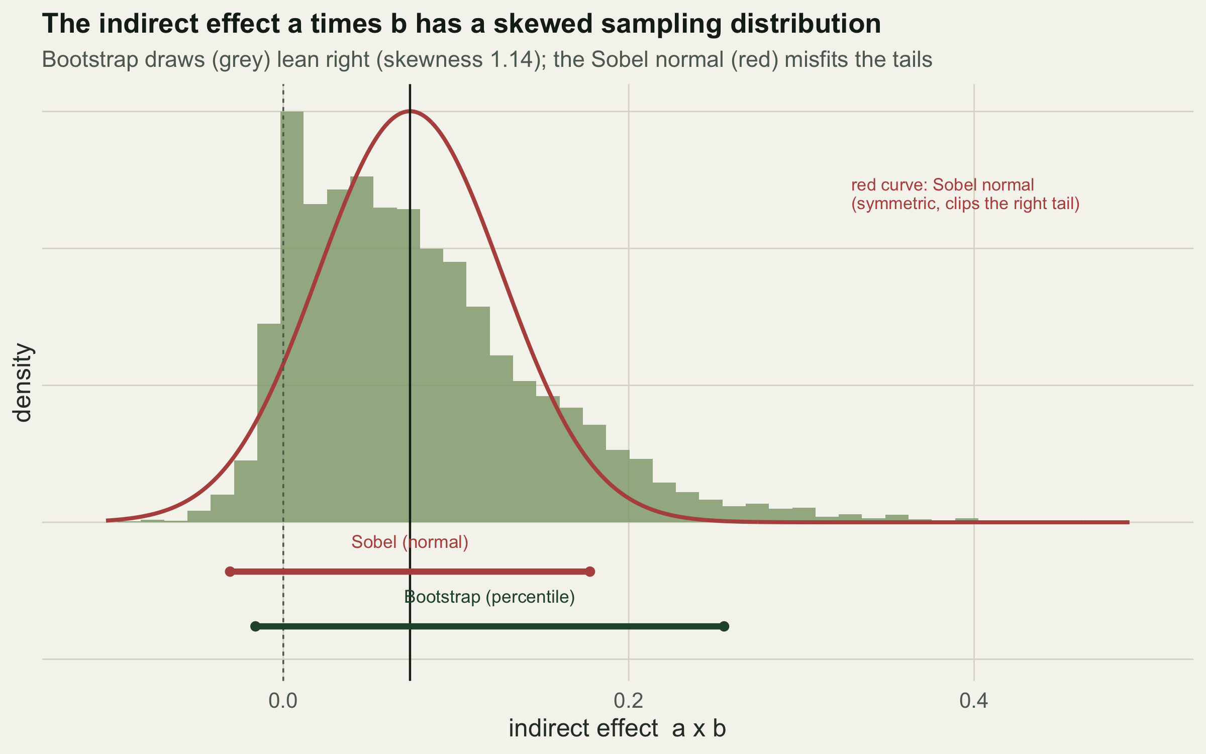

Figure 1

Which interval keeps its promise

A single dataset shows the shapes differ; it cannot show which interval is right. For that, simulate many studies from the same truth, build both 95% intervals for each, and count how often each contains the real indirect effect of 0.122. An honest 95% interval should catch it about 95% of the time.

set.seed(31557)
nsim <- 800; B <- 600
cov_sob <- 0L; cov_bt <- 0L
w_sob <- numeric(nsim); w_bt <- numeric(nsim)
for (s in seq_len(nsim)) {
  xs <- rnorm(n)
  ms <- a_t * xs + sqrt(1 - a_t^2) * rnorm(n)
  ys <- cp_t * xs + b_t * ms + rnorm(n)
  f  <- med_fit(xs, ms, ys)
  lo <- unname(f["indirect"]) - 1.96 * unname(f["sobelSE"])
  hi <- unname(f["indirect"]) + 1.96 * unname(f["sobelSE"])
  w_sob[s] <- hi - lo
  if (ind_true >= lo && ind_true <= hi) cov_sob <- cov_sob + 1L
  bb  <- boot_ind(xs, ms, ys, B)
  blo <- unname(quantile(bb, 0.025)); bhi <- unname(quantile(bb, 0.975))
  w_bt[s] <- bhi - blo
  if (ind_true >= blo && ind_true <= bhi) cov_bt <- cov_bt + 1L
}
cov_sob <- 100 * cov_sob / nsim
cov_bt  <- 100 * cov_bt / nsim

Over 800 simulated studies, the Sobel interval covers the truth 91.8% of the time, short of its nominal 95%. The bootstrap percentile interval covers 94.4%, close to the mark. The two intervals are almost the same average width (0.294 for Sobel, 0.303 for the bootstrap), so the bootstrap is not simply buying coverage by being wider; it is placing the same width in a better position, following the skew instead of straddling it symmetrically.

cv <- data.frame(method = factor(c("Sobel (normal)", "Bootstrap (percentile)"),
                                 levels = c("Sobel (normal)", "Bootstrap (percentile)")),
                 coverage = c(cov_sob, cov_bt), width = c(mean(w_sob), mean(w_bt)))
ggplot(cv, aes(method, coverage, fill = method)) +
  geom_hline(yintercept = 95, colour = te$ink, linetype = "22", linewidth = 0.5) +
  geom_col(width = 0.55) +
  geom_text(aes(label = sprintf("%.1f%%", coverage)), vjust = -0.6, size = 3.8, colour = te$body) +
  geom_text(aes(label = sprintf("mean width\n%.3f", width)), y = 46, size = 3.0,
            colour = te$paper, lineheight = 0.9) +
  annotate("text", x = Inf, y = 95, label = "nominal 95%", colour = te$ink, size = 3.0,
           hjust = 1.05, vjust = -0.5) +
  scale_fill_manual(values = c(`Sobel (normal)` = te$warm, `Bootstrap (percentile)` = te$forest),
                    guide = "none") +
  coord_cartesian(ylim = c(0, 100)) +
  labs(title = sprintf("Coverage of nominal 95%% intervals over %d simulated studies", nsim),
       subtitle = sprintf("n = %d per study, true indirect = %.3f; the Sobel interval undercovers", n, ind_true),
       x = NULL, y = "actual coverage (%)") +
  theme_te(12)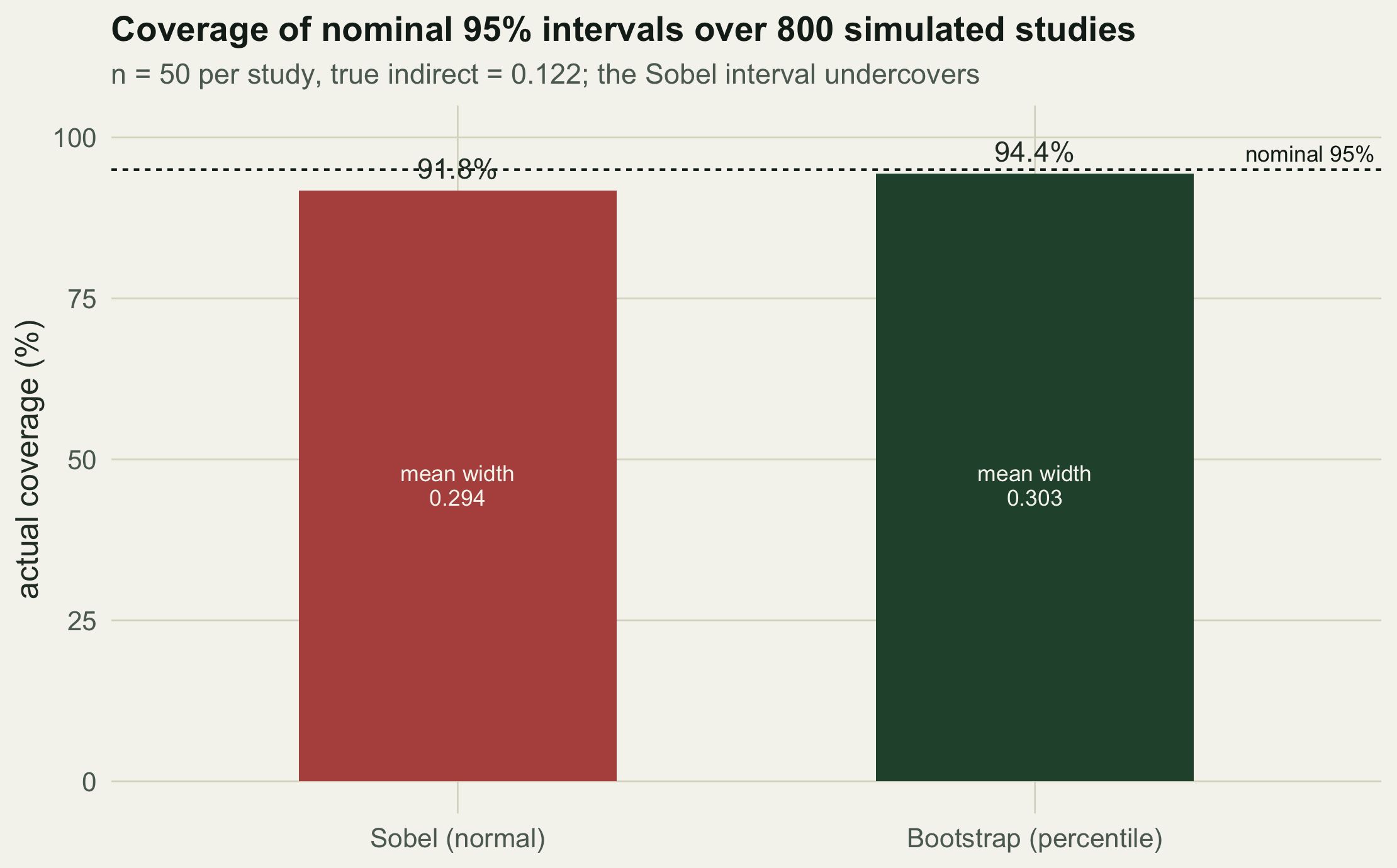

Figure 2

Practical notes

Three caveats keep this in proportion. The bootstrap needs enough resamples: a few thousand for a stable percentile interval, and more if you want the bias-corrected and accelerated variant, which sharpens coverage further at the cost of more computation. The percentile interval used here is the simplest resampling option and already recovers most of what Sobel loses. Next, none of this rescues a genuinely small indirect effect: with fifty observations and a true value near 0.122, both intervals include zero in many samples, so the honest conclusion is often that the mediation is real but imprecisely estimated. A better interval reports that uncertainty faithfully; it does not conjure precision that is not there.

The last caveat is the deepest. A confidence interval for a times b that excludes zero establishes that an indirect association exists under the assumed diagram. It does not establish that the mediator causes the response rather than the reverse, nor that no unmeasured variable drives both. The arrows are still an assumption, and a well-placed interval on the wrong diagram is still wrong. Testing the structure itself, and confronting its limits, is where this series ends.

References

Baron, R. M. and Kenny, D. A. (1986). The moderator-mediator variable distinction in social psychological research: conceptual, strategic, and statistical considerations. Journal of Personality and Social Psychology 51(6): 1173-1182. DOI: 10.1037/0022-3514.51.6.1173

MacKinnon, D. P., Lockwood, C. M., Hoffman, J. M., West, S. G. and Sheets, V. (2002). A comparison of methods to test mediation and other intervening variable effects. Psychological Methods 7(1): 83-104. DOI: 10.1037/1082-989X.7.1.83

MacKinnon, D. P., Lockwood, C. M. and Williams, J. (2004). Confidence limits for the indirect effect: distribution of the product and resampling methods. Multivariate Behavioral Research 39(1): 99-128. DOI: 10.1207/s15327906mbr3901_4

Preacher, K. J. and Hayes, A. F. (2008). Asymptotic and resampling strategies for assessing and comparing indirect effects in multiple mediator models. Behavior Research Methods 40(3): 879-891. DOI: 10.3758/BRM.40.3.879

Sobel, M. E. (1982). Asymptotic confidence intervals for indirect effects in structural equation models. Sociological Methodology 13: 290-312. DOI: 10.2307/270723

Related tutorials

• Path analysis: direct, indirect, and total effects
• Piecewise SEM and the test of d-separation
• Checking a structural equation model
• Bootstrap confidence intervals from scratch

References

Baron RM, Kenny DA 1986 Journal of Personality and Social Psychology 51(6):1173-1182 (10.1037/0022-3514.51.6.1173)
MacKinnon DP, Lockwood CM, Hoffman JM, West SG, Sheets V 2002 Psychological Methods 7(1):83-104 (10.1037/1082-989X.7.1.83)
MacKinnon DP, Lockwood CM, Williams J 2004 Multivariate Behavioral Research 39(1):99-128 (10.1207/s15327906mbr3901_4)
Preacher KJ, Hayes AF 2008 Behavior Research Methods 40(3):879-891 (10.3758/BRM.40.3.879)
Sobel ME 1982 Sociological Methodology 13:290-312 (10.2307/270723)