Checking an empirical dynamic model

Three diagnostics for EDM on systems where the truth is known: series length, shared drivers, and synchrony. What convergent cross mapping catches, and what it cannot.

The three previous posts each ended with a warning. This one takes the warnings seriously and runs the method on systems where the answer is written in the equations, so every claim can be scored.

The order matters. Simplex projection asks whether there is deterministic structure; the S-map measures state dependence and can hand you interaction coefficients; convergent cross mapping turns the reconstruction into a directional causal test. Each step adds an assumption, and this post is about what happens when one fails.

Three checks, three known-truth systems, and one recurring theme: rho is not the evidence. The rise in rho is the evidence, and there is a regime where even that goes quiet.

make_block <- function(x, E, tau = 1) {
  n <- length(x)
  tt <- seq((E - 1) * tau + 1, n)
  M <- matrix(NA_real_, nrow = length(tt), ncol = E)
  for (j in seq_len(E)) M[, j] <- x[tt - (j - 1) * tau]
  list(M = M, t = tt)
}

ccm_once <- function(from, to, E, lib_size, theiler = 0) {
  bl <- make_block(from, E); M <- bl$M; tt <- bl$t
  yv <- to[tt]; n <- length(tt)
  lib <- sample.int(n, min(lib_size, n))
  D <- as.matrix(dist(M))
  pr <- rep(NA_real_, n)
  for (i in seq_len(n)) {
    cand <- lib[lib != i & abs(tt[lib] - tt[i]) > theiler]
    if (length(cand) < E + 1) next
    d <- D[i, cand]
    o <- order(d)[seq_len(E + 1)]
    dn <- d[o]
    w <- if (dn[1] == 0) as.numeric(dn == 0) else exp(-dn / dn[1])
    pr[i] <- sum(pmax(w, 1e-8) * yv[cand[o]]) / sum(pmax(w, 1e-8))
  }
  k <- !is.na(pr)
  suppressWarnings(cor(pr[k], yv[k]))
}

## the reportable statistic: skill at a small library, at a large one, and the rise
ccm_delta <- function(from, to, E, L_lo, L_hi, reps = 20) {
  lo <- mean(replicate(reps, ccm_once(from, to, E, L_lo)), na.rm = TRUE)
  hi <- mean(replicate(reps, ccm_once(from, to, E, L_hi)), na.rm = TRUE)
  c(lo = lo, hi = hi, delta = hi - lo)
}

## Ebisuzaki surrogate: same power spectrum, phases randomised, determinism gone
surrogate_ebi <- function(x) {
  n <- length(x); xm <- mean(x); z <- x - xm
  f <- fft(z); amp <- Mod(f); nyq <- floor(n / 2)
  newf <- complex(modulus = amp, argument = 0)
  newf[2:nyq] <- complex(modulus = amp[2:nyq], argument = runif(nyq - 1, 0, 2 * pi))
  newf[n:(n - nyq + 2)] <- Conj(newf[2:nyq])
  newf[1] <- f[1]
  if (n %% 2 == 0)
    newf[nyq + 1] <- complex(modulus = amp[nyq + 1],
                             argument = ifelse(runif(1) < 0.5, 0, pi))
  Re(fft(newf, inverse = TRUE)) / n + xm
}

Check 1: is the series long enough to show convergence?

Convergence is a statement about what happens as the library fills in. A short series has no room for the comparison: the smallest usable library and the largest are nearly the same library.

The system is the familiar one, X driving Y at strength 0.10. The truth never changes; only the number of observations does. For each length, compare the observed rise against 100 phase-randomised surrogates of X, which keep its spectrum and destroy its trajectory.

set.seed(4267)
lengths <- c(30, 50, 100, 200, 400)
len_res <- do.call(rbind, lapply(lengths, function(nn) {
  d <- gen_coupled(nn)
  L_lo <- 20; L_hi <- nn - 5
  obs <- ccm_delta(d$y, d$x, E = 2, L_lo, L_hi, reps = 30)
  null <- replicate(50, ccm_delta(d$y, surrogate_ebi(d$x), E = 2,
                                  L_lo, L_hi, reps = 5)["delta"])
  data.frame(n = nn, rho_hi = obs["hi"], delta = obs["delta"],
             q95 = quantile(null, 0.95),
             verdict = ifelse(obs["delta"] > quantile(null, 0.95),
                              "convergent", "not convergent"))
}))
rownames(len_res) <- NULL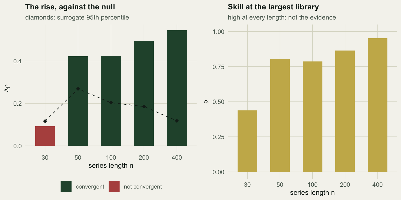

Figure 1: Observed rise in cross-map skill against series length, with the 95th percentile of the surrogate null. The coupling is identical at every length; only the ability to demonstrate it changes.

At n = 30 the rise is +0.092 against a null threshold of +0.116: not convergent. The coupling is there, and the data cannot show it. By n = 50 the rise is +0.421 against +0.268, and every longer series is clearer still.

The right panel is the trap. Cross-map skill at the largest available library is 0.44 even for the thirty-point series, which is a respectable-looking number produced by a test with no power.

Two things go wrong at once at that length, and they are worth separating. With n = 30 the libraries being compared are 20 and 25 points: there is almost no range to converge over, so both the observed rise and the null’s collapse toward zero, and the test has nothing to work with. Then, as the series grows, the null threshold itself falls, from +0.268 at n = 50 to +0.118 at n = 400, because a short library lets autocorrelation manufacture a rise on its own. The observed rise climbs over the same range, from +0.421 to +0.544. The gap opens from both ends, which is why the method feels transformative at n = 400 and useless at n = 30.

Thirty annual counts is a completely ordinary ecological time series. This method cannot do anything with it, and it will not tell you so unless you run the null.

Check 2: is something else driving both?

Two species that never interact, both forced by the same chaotic environmental variable, which enters their dynamics rather than being copied into their abundances.

gen_shared <- function(n, burn = 500, rz = 3.8, ra = 3.7, rb = 3.6,
                       bz1 = 0.5, bz2 = 0.4) {
  N <- n + burn
  z <- numeric(N); a <- numeric(N); b <- numeric(N)
  z[1] <- 0.5; a[1] <- 0.4; b[1] <- 0.35
  for (t in 1:(N - 1)) {
    z[t + 1] <- rz * z[t] * (1 - z[t])                    # driver, autonomous
    a[t + 1] <- a[t] * (ra - ra * a[t] - bz1 * z[t])      # a feels z only
    b[t + 1] <- b[t] * (rb - rb * b[t] - bz2 * z[t])      # b feels z only
  }
  data.frame(z = z[(burn + 1):N], a = a[(burn + 1):N], b = b[(burn + 1):N])
}

set.seed(4267)
ds <- gen_shared(400)
r_ab <- cor(ds$a, ds$b)

ab <- ccm_delta(ds$a, ds$b, E = 2, 20, 399, reps = 30)   # tests b -> a : FALSE
az <- ccm_delta(ds$a, ds$z, E = 2, 20, 399, reps = 30)   # tests z -> a : TRUE
null_ab <- replicate(60, ccm_delta(ds$a, surrogate_ebi(ds$b), E = 2,
                                   20, 399, reps = 5)["delta"])
q95_ab <- quantile(null_ab, 0.95)
p_ab <- mean(null_ab >= ab["delta"])

The two species correlate at 0.52, which on its own would start an argument about competition. The cross map “A xmap B”, which tests whether B drives A, reaches 0.500 at the full library. Reported as a single number, that is a link.

It is not a link. The rise across library lengths is +0.048, against a surrogate null whose 95th percentile is +0.104 and a p-value of 0.22. The true driver, tested the same way, gives a rise of +0.491 and reaches 0.939.

Figure 2: A shared driver produces a moderate cross-map skill between two species that never interact. The convergence test separates it from the real driver link; the skill value alone does not.

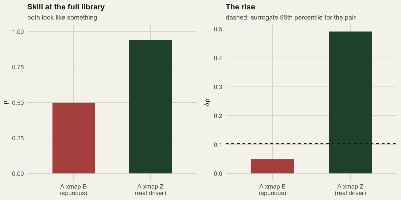
So the procedure works, and it works because of the part that is easy to skip. A cross-map skill of 0.50 between two species with no link between them is exactly the false positive that CCM is accused of producing, and the accusation lands only against the version of the method that reports rho at one library length.

Two caveats keep this from being a clean win. The driver here is strong, chaotic and enters both species the same way; other confounding structures are less kind. And this test only ever had a chance because the driver was measured: had z gone unrecorded, nothing in the two-species analysis would have hinted that a third variable existed. The check is therefore not “run the surrogate test”, it is “run the surrogate test and think hard about what you did not measure”.

Check 3: are the species synchronised?

Now the case that defeats the procedure. Strictly unidirectional forcing: X is autonomous, a logistic map that nothing can influence. Y is forced by X. The reverse link is not weak, it is absent by construction, at every forcing strength.

gen_uni <- function(n, burn = 500, rx = 3.8, ry = 3.5, byx) {
  N <- n + burn; x <- numeric(N); y <- numeric(N); x[1] <- 0.4; y[1] <- 0.2
  for (t in 1:(N - 1)) {
    x[t + 1] <- rx * x[t] * (1 - x[t])                 # nothing enters x. ever.
    y[t + 1] <- y[t] * (ry - ry * y[t] - byx * x[t])
  }
  data.frame(x = x[(burn + 1):N], y = y[(burn + 1):N])
}

set.seed(4267)
strengths <- c(0.1, 2.0)
syn <- do.call(rbind, lapply(strengths, function(s) {
  d <- gen_uni(300, byx = s)
  tr <- ccm_delta(d$y, d$x, E = 2, 20, 299, reps = 20)   # TRUE  : x -> y
  fa <- ccm_delta(d$x, d$y, E = 2, 20, 299, reps = 20)   # FALSE : y -> x
  data.frame(byx = s, r = cor(d$x, d$y),
             true_hi = tr["hi"], true_d = tr["delta"],
             false_hi = fa["hi"], false_d = fa["delta"])
}))
rownames(syn) <- NULL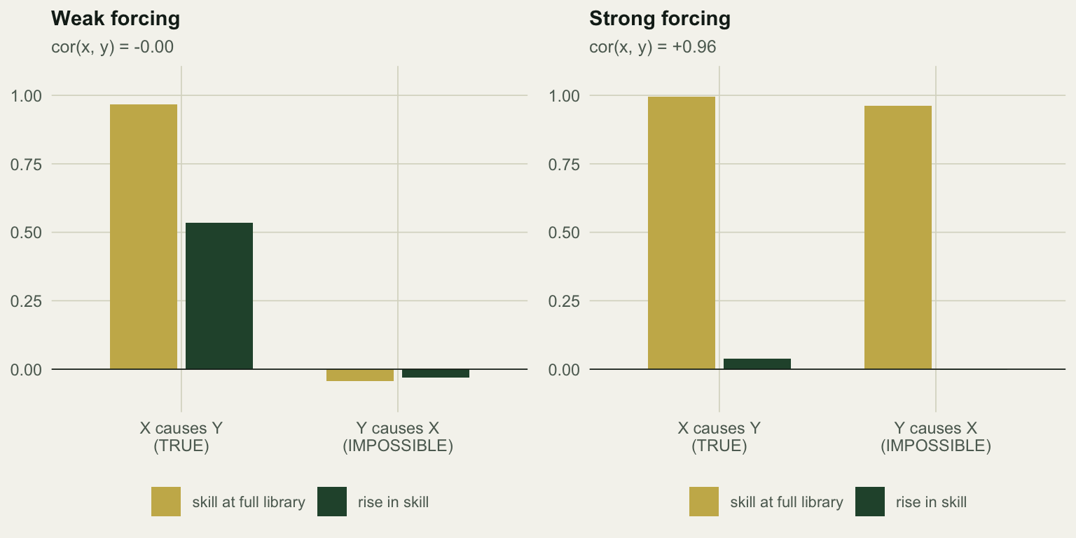

Figure 3: Weak and strong unidirectional forcing. Under weak forcing the test recovers the true direction and rejects the impossible one. Under strong forcing both directions run at high skill and neither converges.

Under weak forcing the method is exemplary. The true direction reaches 0.966 with a rise of +0.534; the impossible direction sits at -0.045 with a rise of -0.031. Correct on both counts, from two series whose correlation is zero to two decimal places.

Turn the forcing up to byx = 2.0 and the two species synchronise: they now correlate at +0.96. Both cross maps are excellent, 0.995 for the true direction and 0.962 for the impossible one. And neither converges: the rises are +0.040 and -0.002.

Read that carefully, because it is worse than a false positive. The convergence criterion refuses the impossible direction, which is right, but it also refuses the true one, which is a strong causal link that dominates the whole system. Applied honestly, the test returns “no evidence of causation in either direction” for a pair of species where one drives the other about as hard as anything drives anything.

The mechanism has a name: generalised synchrony. When the forcing is strong enough, Y’s state becomes a function of X’s state, the two attractors collapse onto what is effectively one manifold, and each series can be recovered from the other with equal ease at any library size. There is nothing left for the library to fill in, so the rise vanishes. The very thing that made the coupling detectable, incomplete determination of one system by the other, is what strong coupling destroys.

The practical diagnostic is the correlation you were told to distrust in the first place. If two species correlate at +0.96 and cross-map each other at over 0.9 already at small libraries, you are probably looking at synchrony, and CCM cannot resolve direction there. A flat curve then means “cannot tell”, not “no link”. Distinguishing the two requires something outside the method: a perturbation, a natural experiment, a mechanistic reason to rule one direction out.

Clark and colleagues hit the same wall from the opposite side, which is worth knowing about because it shows the failure has two faces. Their convergence rule asks whether the rise in skill is reliably above zero rather than whether it beats a spectrum-preserving null, and under strong unidirectional forcing that rule reports causation in both directions instead of neither. Same phenomenon, opposite verdict: how synchrony breaks the test depends on how strict your convergence rule is, and neither verdict is the truth. They also describe the signature to look for, a steep climb over the first few library sizes followed by a long plateau, and one partial escape: where the synchrony comes from a shared external driver rather than from the coupling itself, differencing the series before analysis can weaken it. That does not help here, because the synchrony is the coupling.

The checklist

Table 1

Check	Ask	What goes wrong
Series length	Are there enough points for small and large libraries to differ?	Under about 50 points the test has no power and says nothing
Convergence	Does skill rise with library length, or is it just high?	A single high rho is the classic false positive
Surrogate null	Does the rise exceed phase-randomised surrogates of the driver?	Autocorrelation alone lifts short cross-map curves
Shared driver	Could an unmeasured variable force both series?	A moderate flat cross map between unlinked species
Synchrony	Do the species correlate strongly and cross-map well at small L?	Flat curves mean ‘cannot tell’, not ‘no link’
Embedding	Do conclusions survive E plus or minus one?	The skill curve is flat, so the argmax is noise
Interaction coefficients	Is the coefficient large enough to drive the prediction?	Weak coefficients fluctuate as noise while predicting well

What EDM is for

Nothing here argues against the method. On the coupled system it recovered a fivefold asymmetry in coupling strength from series correlating at 0.11, which no linear tool can do. On the chaotic Ricker it separated determinism from red noise with an identical autocorrelation function. Those are real results and they are not available elsewhere.

The pattern in the failures is consistent. EDM breaks when the geometry it depends on stops being informative: too few points to populate the attractor, an unmeasured variable that puts both species on the same manifold, or coupling so strong that two manifolds become one. In each case the method’s output stays confident and well behaved. It is the shape of the evidence that changes, not its appearance, which is why the checks have to be run rather than assumed.

A working rule: report the curve, not the number; test the rise against a spectrum-preserving surrogate; state the length of your series next to the claim; and treat a flat curve as ambiguous until you have ruled out synchrony. If that sounds like a lot of hedging for one arrow between two species, it is worth remembering what the arrow is being asked to do, which is to establish causation from observation alone.

References

Sugihara, May, Ye, Hsieh, Deyle, Fogarty & Munch 2012 Science 338(6106):496-500 (10.1126/science.1227079)

Cobey & Baskerville 2016 PLoS ONE 11(12):e0169050 (10.1371/journal.pone.0169050)

Ye, Deyle, Gilarranz & Sugihara 2015 Scientific Reports 5:14750 (10.1038/srep14750)

Takens 1981 Lecture Notes in Mathematics 898:366-381 (10.1007/BFb0091924)

Chang, Ushio & Hsieh 2017 Ecological Research 32(6):785-796 (10.1007/s11284-017-1469-9)

Clark, Ye, Isbell, Deyle, Cowles, Tilman & Sugihara 2015 Ecology 96(5):1174-1181 (10.1890/14-1479.1)

Ebisuzaki 1997 Journal of Climate 10(9):2147-2153

Related tutorials

• Convergent cross mapping in ecology
• Simplex projection and delay embedding
• The S-map and state-dependent dynamics
• Checking a time-series model