Checking a time series model

Diagnosing a fitted time series model in base R: residual whiteness with the Ljung-Box test and residual ACF, prewhitening before cross-correlation, and why passing every check still cannot prove a model right.

The three previous posts built time series tools: the correlogram and effective sample size, ARIMA fitting and forecasting, and the periodogram. Each ended on the same warning, that the method is easy to fool. This closing post is about the discipline that keeps them honest: checking. A fitted time series model earns trust only after its residuals are shown to be white, its cross-correlations survive prewhitening, and its forecasts stay calibrated out of sample. We work through the two diagnostics that catch the most mistakes, then set out the full checklist, and finish on the limit that governs all of it: these checks can prove a model wrong, but never prove it right.

Everything is base stats: arima, Box.test, acf, ccf, filter.

Residual whiteness: did the model absorb the autocorrelation?

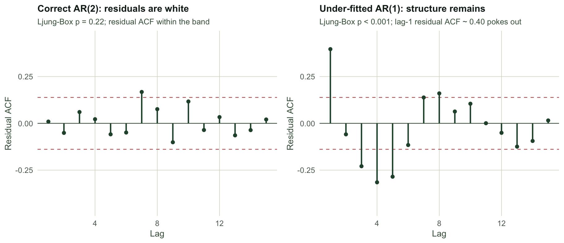
The whole point of an autoregressive model is to soak up the temporal dependence, leaving residuals that are indistinguishable from white noise. If structure remains in the residuals, the model has missed something. We fit two models to the same AR(2) series, the correct one and a deliberately under-fitted AR(1), and inspect what each leaves behind.

set.seed(4243)
phi1 <- 1.2; phi2 <- -0.6; n <- 200
y <- as.numeric(arima.sim(list(ar = c(phi1, phi2)), n = n, sd = 1))

fit_ok <- arima(y, order = c(2, 0, 0))    # correct
fit_un <- arima(y, order = c(1, 0, 0))    # under-fitted
res_ok <- residuals(fit_ok); res_un <- residuals(fit_un)

# Ljung-Box portmanteau test; fitdf subtracts the estimated AR parameters
lb_ok <- Box.test(res_ok, lag = 15, type = "Ljung-Box", fitdf = 2)
lb_un <- Box.test(res_un, lag = 15, type = "Ljung-Box", fitdf = 1)
band <- 1.96 / sqrt(n)
acf_ok <- as.numeric(acf(res_ok, lag.max = 15, plot = FALSE)$acf)[-1]
acf_un <- as.numeric(acf(res_un, lag.max = 15, plot = FALSE)$acf)[-1]

Two complementary tools read the residuals. The residual ACF is the visual check: for a good model every spike should sit inside the band, since white noise has no autocorrelation. The Ljung-Box test is the formal summary, pooling the first several residual autocorrelations into one portmanteau statistic and testing whether they are jointly zero; a small p-value means leftover structure. The results are unambiguous. The correct AR(2) leaves white residuals: its Ljung-Box p-value is 0.22 and 1 of 15 residual autocorrelations stray past the band, about what chance alone produces. The under-fitted AR(1) fails both: its Ljung-Box statistic is 102 with a p-value below 0.001, and 5 residual autocorrelations break the band, the largest 0.40 at lag 1, the exact structure a first-order model cannot represent.

Figure 1: Residual ACF after fitting. Left: the correct AR(2) leaves white residuals, every spike inside the band and Ljung-Box comfortably non-significant. Right: the under-fitted AR(1) leaves a strong lag-1 residual autocorrelation and a decisive Ljung-Box rejection.

Prewhitening before you cross-correlate

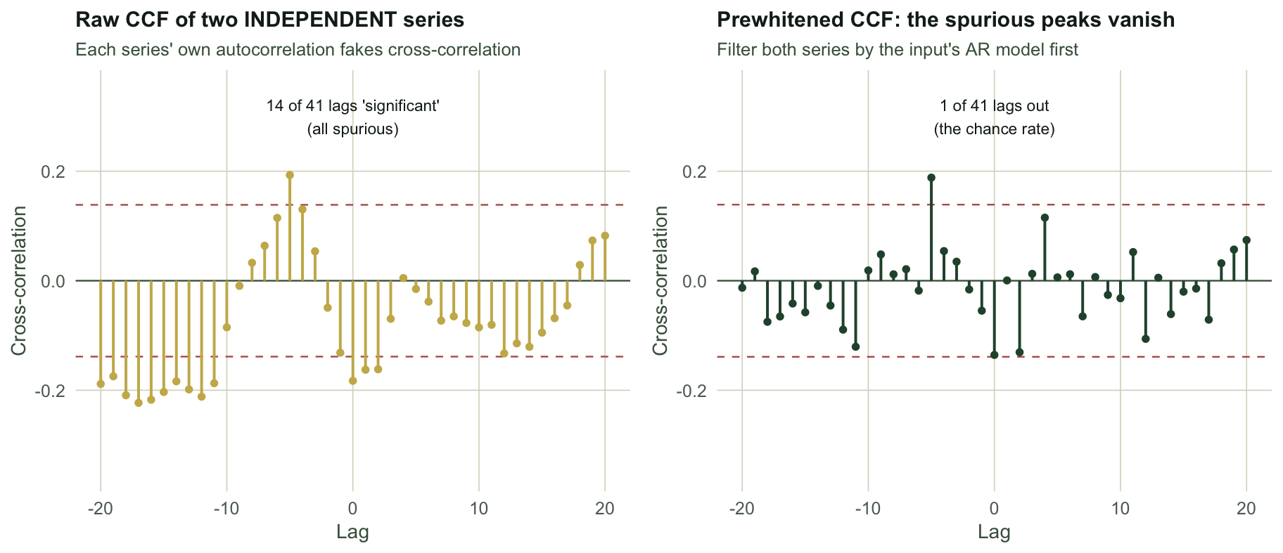
The first post showed that two independent series can look correlated simply because each is autocorrelated. The same trap is worse for the cross-correlation function, the CCF, which many ecologists reach for to find lagged relationships, whether a predator tracking prey or a population lagging a climate driver. The raw CCF between two persistent series is riddled with spurious peaks, because each series’ own autocorrelation smears across every lag. The Box-Jenkins remedy is prewhitening: filter the input series by its own fitted autoregressive model so it becomes white, apply the identical filter to the output series, and only then compute the CCF. We demonstrate on two series generated independently.

set.seed(51)
x <- as.numeric(arima.sim(list(ar = 0.7), n = n))
z <- as.numeric(arima.sim(list(ar = 0.7), n = n))    # generated independently of x

cc_raw <- ccf(x, z, lag.max = 20, plot = FALSE)      # raw, misleading
raw_sig <- sum(abs(cc_raw$acf) > band)

ar_x <- arima(x, order = c(1, 0, 0))                 # fit the input's AR model
phx <- coef(ar_x)["ar1"]
xw <- residuals(ar_x)                                # prewhitened input (white)
zw <- z[-1] - phx * z[-length(z)]                    # SAME filter applied to output
cc_pw <- ccf(xw[-1], zw, lag.max = 20, plot = FALSE)
b_pw <- 1.96 / sqrt(length(zw))
pw_sig <- sum(abs(cc_pw$acf) > b_pw)

The raw CCF flags 14 of its 41 lags as significant, every one of them an artefact of two independent series. After prewhitening, only 1 lag steps past the band, exactly the false-positive rate chance would give across that many lags. The lesson from the correlogram post carries over intact: before reading any cross-correlation between two time series, prewhiten, or the autocorrelation each series already carries will invent a relationship that is not there.

Figure 2: Cross-correlation of two independent series. Left: the raw CCF shows many peaks past the band, all spurious, produced by each series’ own autocorrelation. Right: after prewhitening, the CCF collapses to noise within the band.

The full checklist

Residual whiteness and prewhitening catch the two commonest errors, but a complete check for an ecological time series model runs wider. Residuals should be white, tested with the residual ACF and a Ljung-Box statistic, and the same residuals should show no trend in their variance and no gross departure from normality if the prediction intervals are to mean anything. Any cross-correlation with a covariate must be read only after prewhitening. Forecasts should be checked out of sample rather than in: hold back the tail of the series, forecast it, and confirm the nominal interval covers close to its stated rate, remembering from the ARIMA post that plug-in intervals run a little narrow even when the model form is right. And where the question is periodicity, the spectral post adds two sanity checks that no residual plot will supply: confirm the sampling interval places any expected cycle below the Nyquist frequency so it cannot be an alias, and judge every periodogram peak against a red-noise null rather than a white one.

What to carry away

Every check in this post is a falsification test. A significant Ljung-Box statistic, a prewhitened CCF peak, an interval that undercovers out of sample: each of these proves a model inadequate. What none of them can do is prove a model correct. A model can leave white residuals and still be the wrong model, because different processes can produce identical second-order structure. An AR(2) with a spectral peak, a genuine driven cycle, and an aliased fast rhythm can all pass a residual check while telling different stories about the ecology. The tests narrow the field of plausible models and eliminate the clearly broken ones, which is exactly what makes them worth running, but the final judgement rests on whether the model’s form matches what is known about the system, not on any single p-value. That is the honest end point of the whole series: diagnostics earn a model the right to be used, they do not certify it true.

Related tutorials

• Temporal autocorrelation and effective sample size
• Fitting ARIMA models to ecological time series
• Spectral analysis of population cycles
• Estimating population trends from monitoring data

References

• Box, Jenkins, Reinsel & Ljung 2015 Time Series Analysis: Forecasting and Control, 5th ed, Wiley, ISBN 978-1-118-67502-1
• Ives, Abbott & Ziebarth 2010 Ecology 91(3):858-871 (10.1890/09-0442.1)
• Ljung & Box 1978 Biometrika 65(2):297-303 (10.1093/biomet/65.2.297)
• Shumway & Stoffer 2017 Time Series Analysis and Its Applications, 4th ed, Springer, ISBN 978-3-319-52451-1